Ensemble Modeling in a Binary Classification Problem in Chinese A-Share Market
2017-11-15
In this research paper we try to use as much information on a stock as we can on Ricequant, to train a robust binary classifier for expected returns on a rolling basis. As an extra, we create a brand-new accuracy metric based on behavioral economics for model traing, which enhanced the fitting of the models (in the language of classical metrics, e.g. accuracy or pricision scores) by 3 to 5 times. The advantage of this new metric will be covered in the corresponding sector.
Section 1: Environment Preparation
First we import the necessary packages we’re going to use later.
%config InlineBackend.figure_format = 'retina'

import numpy as np
import pandas as pd
from scipy.special import logit
from datetime import datetime
from dateutil.relativedelta import relativedelta
from tech import technical
import warnings
warnings.filterwarnings('ignore')

import matplotlib.pyplot as plt
import seaborn as sns

from xgboost import XGBClassifier
from sklearn.decomposition import PCA, KernelPCA
from sklearn.cross_validation import KFold, cross_val_score
from sklearn.metrics import make_scorer, accuracy_score, precision_score, recall_score
from sklearn.grid_search import GridSearchCV
from sklearn.feature_selection import VarianceThreshold, RFE, SelectKBest, chi2
from sklearn.preprocessing import MinMaxScaler
from sklearn.pipeline import Pipeline, FeatureUnion
from sklearn.linear_model import LogisticRegression
from sklearn.discriminant_analysis import LinearDiscriminantAnalysis
from sklearn.neighbors import KNeighborsClassifier
from sklearn.tree import DecisionTreeClassifier
from sklearn.naive_bayes import GaussianNB
from sklearn.svm import SVC
from sklearn.ensemble import BaggingClassifier, ExtraTreesClassifier, GradientBoostingClassifier, VotingClassifier, RandomForestClassifier, AdaBoostClassifier

sns.set_style('whitegrid')
pd.set_option('display.max_columns', None) # display all columns
Global configurations.
pool = index_components('000050.XSHG')
window = 3  # use the past 6 months for training and testing
risk_preference = -0.2  # in the range of (-1,1) exclusive!
verbose = True  # set to False when you don't want to waste time on plotting
Section 2: Data Preparation
Load the raw data and encapsulate into a Pandas panel.
today = datetime.today()
s = pool[11]
price_df = get_price(s,today-relativedelta(months=window+6),today-relativedelta(days=1),'1d',['open','close','high','low','volume'])
price_df['mkt'] = get_price('000300.XSHG',today-relativedelta(months=window+6),today-relativedelta(days=1),'1d',['close'])
X_ = pd.DataFrame(technical(price_df),index=price_df.index,columns=np.arange(78).astype('str')).ix[-window*20-1:,:]
Some further data investigation.
Unshifted data for training:
for f in range(17,78): X_.ix[:,f] = X_.ix[:,f].astype('category')
y_ = (price_df.ix[X_.index,'close'] > price_df.ix[X_.index,'open']).astype('int')
Shift the data so that they corresponds with
$$ y_i = \text{clf}(X_i). $$
X = X_.ix[:-1,:]
y = y_[1:]
print(X.shape)
print(y.shape)
print(y.value_counts())
(60, 78)
(60,)
1    32
0    28
dtype: int64
y.describe()
count    60.000000
mean      0.533333
std       0.503098
min       0.000000
25%       0.000000
50%       1.000000
75%       1.000000
max       1.000000
dtype: float64
X.describe(include=['number'])
| 0 | 1 | 2 | 3 | 4 | 5 | 6 | 7 | 8 | 9 | 10 | 11 | 12 | 13 | 14 | 15 | 16 | |
|---|---|---|---|---|---|---|---|---|---|---|---|---|---|---|---|---|---|
| count | 60.000000 | 60.000000 | 60.000000 | 60.000000 | 60.000000 | 60.000000 | 60.000000 | 60.000000 | 60.000000 | 60.000000 | 60.000000 | 60.000000 | 60.000000 | 60.000000 | 6.000000e+01 | 60.000000 | 60.000000 |
| mean | 0.976212 | 25.990400 | 25.656650 | 24.940308 | 22.879636 | 21.834747 | 20.977319 | 39.063571 | 35.434052 | 0.852667 | 67.581394 | 26.807436 | 25.990400 | 25.173364 | 1.039211e+09 | 0.723869 | 24.547501 |
| std | 0.015776 | 2.827868 | 2.770969 | 2.614787 | 1.668471 | 1.437906 | 1.220115 | 7.954479 | 7.286649 | 0.354867 | 7.811732 | 3.090838 | 2.827868 | 2.616494 | 1.263014e+08 | 0.168018 | 4.961348 |
| min | 0.948008 | 22.640000 | 22.085000 | 21.392000 | 20.650167 | 19.762876 | 19.285863 | 25.863478 | 26.096620 | 0.413193 | 54.834433 | 22.887871 | 22.640000 | 22.083778 | 8.750972e+08 | 0.527858 | 16.936824 |
| 25% | 0.965606 | 23.293000 | 23.043000 | 22.981875 | 21.499667 | 20.572173 | 19.949996 | 32.360567 | 27.708563 | 0.528046 | 61.687466 | 23.800034 | 23.293000 | 22.799033 | 9.242619e+08 | 0.578824 | 20.770453 |
| 50% | 0.974243 | 25.244000 | 24.591000 | 24.007250 | 22.387833 | 21.624111 | 20.712315 | 39.207117 | 34.467175 | 0.749777 | 66.749465 | 26.030462 | 25.244000 | 24.397322 | 1.038170e+09 | 0.656475 | 23.760415 |
| 75% | 0.987142 | 29.210500 | 28.633250 | 27.278500 | 24.174250 | 23.017472 | 21.933203 | 46.661330 | 41.646060 | 1.179799 | 73.758827 | 30.086332 | 29.210500 | 27.848188 | 1.159543e+09 | 0.852259 | 27.627880 |
| max | 1.007653 | 30.286000 | 29.820000 | 29.691500 | 26.243333 | 24.528111 | 23.411667 | 49.526365 | 46.601986 | 1.427553 | 82.767827 | 31.203224 | 30.286000 | 29.442553 | 1.301344e+09 | 1.065128 | 35.042981 |
X.describe(include=['category'])
| 17 | 18 | 19 | 20 | 21 | 22 | 23 | 24 | 25 | 26 | 27 | 28 | 29 | 30 | 31 | 32 | 33 | 34 | 35 | 36 | 37 | 38 | 39 | 40 | 41 | 42 | 43 | 44 | 45 | 46 | 47 | 48 | 49 | 50 | 51 | 52 | 53 | 54 | 55 | 56 | 57 | 58 | 59 | 60 | 61 | 62 | 63 | 64 | 65 | 66 | 67 | 68 | 69 | 70 | 71 | 72 | 73 | 74 | 75 | 76 | 77 | |
|---|---|---|---|---|---|---|---|---|---|---|---|---|---|---|---|---|---|---|---|---|---|---|---|---|---|---|---|---|---|---|---|---|---|---|---|---|---|---|---|---|---|---|---|---|---|---|---|---|---|---|---|---|---|---|---|---|---|---|---|---|---|
| count | 60.0 | 60.0 | 60.0 | 60.0 | 60.0 | 60.0 | 60.0 | 60.0 | 60.0 | 60.0 | 60.0 | 60.0 | 60.0 | 60.0 | 60.0 | 60.0 | 60.0 | 60.0 | 60.0 | 60.0 | 60.0 | 60.0 | 60.0 | 60.0 | 60.0 | 60.0 | 60.0 | 60.0 | 60.0 | 60.0 | 60.0 | 60.0 | 60.0 | 60.0 | 60.0 | 60.0 | 60.0 | 60.0 | 60.0 | 60.0 | 60.0 | 60.0 | 60.0 | 60.0 | 60.0 | 60.0 | 60.0 | 60.0 | 60.0 | 60.0 | 60.0 | 60.0 | 60.0 | 60.0 | 60.0 | 60.0 | 60.0 | 60.0 | 60.0 | 60.0 | 60.0 |
| unique | 1.0 | 1.0 | 1.0 | 2.0 | 2.0 | 1.0 | 1.0 | 1.0 | 2.0 | 3.0 | 1.0 | 3.0 | 1.0 | 1.0 | 2.0 | 2.0 | 1.0 | 1.0 | 3.0 | 1.0 | 1.0 | 1.0 | 2.0 | 2.0 | 2.0 | 3.0 | 3.0 | 3.0 | 4.0 | 1.0 | 2.0 | 1.0 | 1.0 | 2.0 | 1.0 | 1.0 | 1.0 | 2.0 | 3.0 | 3.0 | 2.0 | 1.0 | 1.0 | 1.0 | 1.0 | 1.0 | 2.0 | 1.0 | 2.0 | 2.0 | 3.0 | 3.0 | 1.0 | 1.0 | 1.0 | 1.0 | 2.0 | 1.0 | 1.0 | 1.0 | 1.0 |
| top | 0.0 | 0.0 | 0.0 | 0.0 | 0.0 | 0.0 | 0.0 | 0.0 | 0.0 | 0.0 | 0.0 | 0.0 | 0.0 | 0.0 | 0.0 | 0.0 | 0.0 | 0.0 | 0.0 | 0.0 | 0.0 | 0.0 | 0.0 | 0.0 | 0.0 | 0.0 | 0.0 | 0.0 | 0.0 | 0.0 | 0.0 | 0.0 | 0.0 | 0.0 | 0.0 | 0.0 | 0.0 | 0.0 | 0.0 | 0.0 | 0.0 | 0.0 | 0.0 | 0.0 | 0.0 | 0.0 | 0.0 | 0.0 | 0.0 | 0.0 | 0.0 | 0.0 | 0.0 | 0.0 | 0.0 | 0.0 | 0.0 | 0.0 | 0.0 | 0.0 | 0.0 |
| freq | 60.0 | 60.0 | 60.0 | 59.0 | 57.0 | 60.0 | 60.0 | 60.0 | 59.0 | 47.0 | 60.0 | 55.0 | 60.0 | 60.0 | 59.0 | 51.0 | 60.0 | 60.0 | 53.0 | 60.0 | 60.0 | 60.0 | 59.0 | 59.0 | 59.0 | 55.0 | 58.0 | 49.0 | 51.0 | 60.0 | 59.0 | 60.0 | 60.0 | 59.0 | 60.0 | 60.0 | 60.0 | 51.0 | 48.0 | 57.0 | 57.0 | 60.0 | 60.0 | 60.0 | 60.0 | 60.0 | 55.0 | 60.0 | 59.0 | 59.0 | 51.0 | 41.0 | 60.0 | 60.0 | 60.0 | 60.0 | 59.0 | 60.0 | 60.0 | 60.0 | 60.0 |
unbalance = sum(y==1)/len(y)
if not (2/5 < unbalance < 3/5): print('Unbalanced dataset!!!')
unbalance
0.53333333333333333
data = X
data.loc[:,'y'] = y.values
data.columns
Index(['0', '1', '2', '3', '4', '5', '6', '7', '8', '9', '10', '11', '12',
       '13', '14', '15', '16', '17', '18', '19', '20', '21', '22', '23', '24',
       '25', '26', '27', '28', '29', '30', '31', '32', '33', '34', '35', '36',
       '37', '38', '39', '40', '41', '42', '43', '44', '45', '46', '47', '48',
       '49', '50', '51', '52', '53', '54', '55', '56', '57', '58', '59', '60',
       '61', '62', '63', '64', '65', '66', '67', '68', '69', '70', '71', '72',
       '73', '74', '75', '76', '77', 'y'],
      dtype='object')
Quick look at the distribution of y.
if verbose:
    ax = plt.axes()
    sns.countplot(x='y', data=data, ax=ax)
    ax.set_title('Actual y Distribution (total: {})'.format(len(data)))
    plt.show()

At first we can see that the target variable is distributed quite equally. We won’t perform any actions to deal with imbalanced dataset. First we present the continuous data using boxplot (described in the following image)
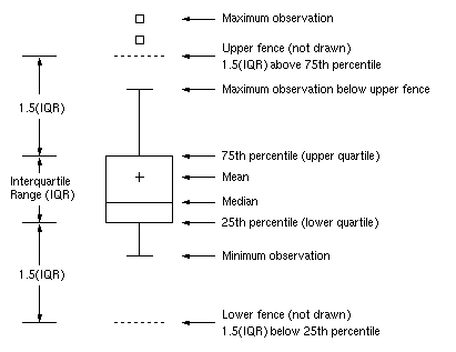
Boxplot of y against continuous variables.
if verbose:
    f, axarr = plt.subplots(4, 4, figsize=(15, 15))

    for i in range(16):
        sns.boxplot(x=str(i), y='y', data=data, showmeans=True, ax=axarr[i//4,i%4])
        axarr[i//4,i%4].set_title('factor '+str(i))

    plt.tight_layout()
    plt.show()

Pairplot of all continous variables.
if verbose:
    sns.pairplot(data, vars=[str(i) for i in range(1,17)], hue='y', size=3)
    plt.show()

Dummy encoding for categorical variables.
for i in range(17,78):
    dummies = pd.get_dummies(data.ix[:,i])
    dummies = dummies.add_prefix("{}#".format(i))
    data.drop(str(i), axis=1, inplace=True)
    data = data.join(dummies)
Section 3: Feature Selection
Drop columns that contains only one value.
mask = data.std() == 0
data_valid = data.ix[:,~mask]
X = data_valid.drop('y', axis=1)
y = data_valid['y']
print(X.columns.tolist())
['0', '1', '2', '3', '4', '5', '6', '7', '8', '9', '10', '11', '12', '13', '14', '15', '16', '19#0.0', '19#100.0', '21#-100.0', '21#0.0', '24#-100.0', '24#0.0', '26#-100.0', '26#0.0', '26#100.0', '28#0.0', '28#100.0', '29#-100.0', '29#0.0', '30#-100.0', '30#0.0', '30#100.0', '31#-200.0', '31#-100.0', '31#0.0', '31#100.0', '32#0.0', '32#100.0', '36#-100.0', '36#0.0', '36#100.0', '37#0.0', '37#100.0', '40#0.0', '40#100.0', '41#0.0', '41#100.0', '42#-100.0', '42#0.0', '42#100.0', '45#-100.0', '45#0.0', '49#0', '49#1', '51#0', '51#1', '53#0', '53#1', '54#0', '54#1', '55#0', '55#1', '56#0', '56#1', '57#0', '57#1', '58#0', '58#1', '59#0', '59#1', '60#0', '60#1', '61#0', '61#1', '62#0', '62#1', '64#0', '64#1', '65#0', '65#1', '66#0', '66#1', '68#0', '68#1', '69#0', '69#1', '70#0', '70#1', '72#0', '72#1', '75#0', '75#1', '76#0', '76#1']
Variance Ranking
vt = VarianceThreshold().fit(X)
ranks = (-vt.variances_).argsort().argsort()
feat_var_threshold = X.columns[ranks<=20]
print(feat_var_threshold.tolist())
['1', '2', '3', '4', '5', '6', '7', '8', '9', '10', '11', '12', '13', '14', '16', '31#0.0', '36#0.0', '42#0.0', '65#0', '70#0', '70#1']
Random Forest
model = RandomForestClassifier()
model.fit(X,y)
feature_imp = pd.DataFrame(model.feature_importances_, index=X.columns, columns=['importance'])
feat_imp_20 = feature_imp.sort_values('importance', ascending=False).head(20).index
print(feat_imp_20.tolist())
['16', '2', '13', '14', '9', '8', '0', '1', '15', '10', '7', '6', '68#0', '70#1', '4', '64#0', '11', '30#0.0', '3', '5']
Chi2 Test
X_minmax = MinMaxScaler([0,1]).fit_transform(X)
X_scored = SelectKBest(score_func=chi2, k='all').fit(X_minmax, y)
feature_scoring = pd.DataFrame({'feature': X.columns,'score': X_scored.scores_})
feat_scored_20 = feature_scoring.sort_values('score', ascending=False).head(20)['feature'].values
print(feat_scored_20.tolist())
['42#-100.0', '64#1', '36#-100.0', '70#0', '68#1', '40#100.0', '31#-100.0', '60#1', '76#1', '51#0', '30#100.0', '32#100.0', '24#-100.0', '21#-100.0', '53#0', '30#-100.0', '57#1', '58#1', '59#1', '62#1']
Recursive Feature Elimination (RFE)
with logistic regression model.
rfe = RFE(LogisticRegression(),20)
rfe.fit(X, y)
feature_rfe_scoring = pd.DataFrame({'feature': X.columns,'score': rfe.ranking_})
feat_rfe_20 = feature_rfe_scoring[feature_rfe_scoring['score'] == 1]['feature'].values
print(feat_rfe_20.tolist())
['1', '2', '3', '4', '5', '6', '7', '8', '10', '11', '12', '13', '14', '16', '36#0.0', '40#0.0', '42#0.0', '68#0', '70#0', '70#1']
Final selection of features
is the union of all previous sets.
features = np.hstack([feat_var_threshold,feat_imp_20,feat_scored_20,feat_rfe_20])
features = np.unique(features)
print('Final features ({} in total): {}'.format(len(features),', '.join(features)))
Final features (46 in total): 0, 1, 10, 11, 12, 13, 14, 15, 16, 2, 21#-100.0, 24#-100.0, 3, 30#-100.0, 30#0.0, 30#100.0, 31#-100.0, 31#0.0, 32#100.0, 36#-100.0, 36#0.0, 4, 40#0.0, 40#100.0, 42#-100.0, 42#0.0, 5, 51#0, 53#0, 57#1, 58#1, 59#1, 6, 60#1, 62#1, 64#0, 64#1, 65#0, 68#0, 68#1, 7, 70#0, 70#1, 76#1, 8, 9
Section 4: Model Training
1. Split the training and testing data (ratio: 3:1).
data_clean = data_valid.ix[:,features.tolist()+['y']]
tot_len = len(data_clean)
split_len = tot_len * 3 // 4
X_train = data_clean.ix[:split_len,features]
X_test = data_clean.ix[split_len:,features]
y_train = data_clean.ix[:split_len,'y']
y_test = data_clean.ix[split_len:,'y']
print('Clean dataset shape: {}'.format(data_clean.shape))
print('Train features shape: {}'.format(X_train.shape))
print('Test features shape: {}'.format(X_test.shape))
print('Train label shape: {}'. format(y_train.shape))
print('Test label shape: {}'. format(y_test.shape))
Clean dataset shape: (60, 47)
Train features shape: (45, 46)
Test features shape: (15, 46)
Train label shape: (45,)
Test label shape: (15,)
2. PCA visualization of training data
PCA plot
if verbose:
    components = 8
    pca = PCA(n_components=components).fit(X_train)
    pca_variance_explained_df = pd.DataFrame({'component': np.arange(1, components+1),'variance_explained': pca.explained_variance_ratio_})
    ax = sns.barplot(x='component', y='variance_explained', data=pca_variance_explained_df)
    ax.set_title('PCA - Variance explained')
    plt.show()

Lmplot
if verbose:
    X_pca = pd.DataFrame(pca.transform(X_train)[:,:2])
    X_pca['target'] = y_train.values
    X_pca.columns = ["x", "y", "target"]
    sns.lmplot('x','y',
               data=X_pca,
               hue="target",
               fit_reg=False,
               markers=["o", "x"],
               palette="Set1",
               size=7,
               scatter_kws={"alpha": .2})
    plt.show()

3. A New Accuracy Metric Based on Utility and Risk-Aversion
Instead of using existing accuracy or error metrics, e.g. accuracy scores and log loss, we tend to come up with our own metric that suits this scenario better. According to classical utility theory, the utility on the expected net return of a transaction should at least follow these properties:
- Higher expected returns means higher utility;
- Zero expected return means zero absolute utility;
- Marginal utility decreases with higher expected returns;
- The utility is robust of scaling.
Mathematically, therefore, we know a well-behaved utility function $U(x)$ has:
- A non-negative first-order derivative;
- A non-positive second-order derivative;
- A zero at
$x=0$.
However, since late 20th century, this setting of utility has been widely criticized and the voice was mainly from behavioral economics. This group of people managed a huge number of empirical experiments and showed how poor such utility models work when the variation of risk-aversion is considered. Risk-aversion was originally introduced to catch the aversion of a human against uncertainty. In classical economics, there are a range of measures to depict such aversion. One of the most famous is Arrow–Pratt measure of absolute risk-aversion (ARA), which is defined based on the utility function:
$$ ARA = -\frac{U^{\prime}(x)}{U^{\prime\prime}(x)}. $$
The Arrow-Pratt absolute risk-aversion is well successful not only because it catches the concavity of the utility, but also it can be expanded into many special cases, mainly w.r.t. different classical utility functions like exponential or hyperbolic absolute utility. However, it is not in line with common sense, pointed by Daniel Kahneman and Amos Tversky in their prospect theory in 1972. The theory has been well further developed since 1992 and is now accepted as a more realistic model for uncertainty perception psychologically.
Different from the classical expected utility theory, the prospect theory specifies the utility in the following four implications:
- Certainty effect: most people are risk-averse about gaining;
- Reflection effect: most people are risk-loving about losing;
- Loss aversion: most people are more sensitive to losses than to gains;
- Reference dependence: most people’s perception of uncertainty is based on the reference point.
Considering here the notion of “most people” is typically based on the fact tha most investors are more or less risk-averse, we simplify the model by giving assumptions as follows:
- The first-order derivative of the utility is non-negative for all outcome;
- For risk-averse investors, the second-order derivative of the utility is non-negative for losses while non-positive for gains;
- For risk-loving investors, the second-order derivative of the utility is non-positive for losses while non-negative for gains;
- For risk-neutral investors, the second-order derivative is zero everywhere
while for the loss aversion implication, we don’t take it into consideration as the influence turned out to be minuscule compared with the loss of model simplicity.
Therefore, with the previous four assumptions, we can easily come up with a nice utility function w.r.t. prediction accuracy:
$$ U(x) = sgn(x-1/2)|2x-1|^{2^{logit\left(\frac{r+1}{2}\right)}} $$
where $sgn(\cdot)$ is the sign function and $logit(\cdot)$ is the logit function, which is also known as the inverse of the sigmoidal “logistic” function:
$$ logit(x)=\ln\left(\frac{x}{1-x}\right). $$
It is easy to validate that our utility follows the configuration and because of its monotonicity and continuity in $[0,1]$, is a well-behaved accuracy metric for further learning algorithms.
Utility Curve
f = lambda x, r: (2*(x>0.5)-1)*abs(2*x-1)**(2**logit((r+1)/2))
if verbose:
    colors = ['red','orange','yellow','lime','cyan']
    r_grid = [-0.9,-0.5,0,0.5,0.9]
    x_grid = np.linspace(0,1,100)
    fig, ax = plt.subplots(figsize=(5,5))
    for i in range(len(r_grid)):
        f_grid = [f(x,r_grid[i]) for x in x_grid]
        ax.plot(x_grid, f_grid,c=colors[i],label='r = {:> 3.1f}'.format(r_grid[i]))
    ax.plot((0,1),(0,0),c='black')
    box = ax.get_position()
    ax.set_position([box.x0, box.y0, box.width * 0.8, box.height])
    ax.legend(loc='center left', bbox_to_anchor=(1, 0.5))
    ax.set_ylim([-1,1])
    ax.set_xlim([0,1])
    plt.xlabel('Accuracy')
    plt.ylabel('Utility')
    plt.title('Utility Curve for Different Risk Preferences')
    plt.show()

def custom_score(y_true, y_pred):
    x = sum(y_pred == y_true) / len(y_true)
    r = risk_preference
    return f(x,r)
seed = 7
processors = 1
num_folds = 4
num_instances = len(X_train)
scoring = make_scorer(custom_score)

kfold = KFold(n=num_instances, n_folds=num_folds, random_state=seed)
First let’s have a quick spot-check.
# Some basic models
models = []
models.append(('LR', LogisticRegression()))
models.append(('LDA', LinearDiscriminantAnalysis()))
models.append(('KNN', KNeighborsClassifier(n_neighbors=5)))
models.append(('DT', DecisionTreeClassifier()))
models.append(('GNB', GaussianNB()))
models.append(('SVC', SVC(probability=True, class_weight='balanced')))

# Evaluate each model in turn
results = []
names = []

for name, model in models:
    cv_results = cross_val_score(model, X_train, y_train, cv=kfold, scoring=scoring, n_jobs=processors)
    results.append(cv_results)
    names.append(name)
    print("{}: ({:.3f}) +/- ({:.3f})".format(name, cv_results.mean(), cv_results.std()))
LR: (0.117) +/- (0.436)
LDA: (0.518) +/- (0.163)
KNN: (0.255) +/- (0.263)
DT: (0.255) +/- (0.263)
GNB: (-0.106) +/- (0.393)
SVC: (0.117) +/- (0.436)
Let’s first look at ensemble results.
Section 5: Ensemble Modeling and Validation
1. Bagging (Bootstrap Aggregation)
Prediction of a bagging model is the average of all sub-models.
Bagged Decision Trees
Bagged Desicion Trees performs the best when the variance is large in the dataset.
cart = DecisionTreeClassifier()
num_trees = 100
model = BaggingClassifier(base_estimator=cart, n_estimators=num_trees, random_state=seed)
results = cross_val_score(model, X_train, y_train, cv=kfold, scoring=scoring, n_jobs=processors)
print("({:.3f}) +/- ({:.3f})".format(results.mean(), results.std()))
(0.158) +/- (0.312)
Random Forest
Random forest is a famous extension to bagged decision trees. It is usually more precise but slower, especially for large number of leaves.
num_trees = 100
num_features = 10
model = RandomForestClassifier(n_estimators=num_trees, max_features=num_features)
results = cross_val_score(model, X_train, y_train, cv=kfold, scoring=scoring, n_jobs=processors)
print("({:.3f}) +/- ({:.3f})".format(results.mean(), results.std()))
(-0.082) +/- (0.295)
Extra Trees
Randomness is introduced to investigate further precision.
num_trees = 100
num_features = 10
model = ExtraTreesClassifier(n_estimators=num_trees, max_features=num_features)
results = cross_val_score(model, X_train, y_train, cv=kfold, scoring=scoring, n_jobs=processors)
print("({:.3f}) +/- ({:.3f})".format(results.mean(), results.std()))
(0.015) +/- (0.484)
2. Boosting Boosting ensembles a sequence of weak learners for better performance.
AdaBoost
AdaBoost simply gives the weighted average of results by a series of weak learners, with updating the weight vector in each iteration.
model = AdaBoostClassifier(n_estimators=100, random_state=seed)
results = cross_val_score(model, X_train, y_train, cv=kfold, scoring=scoring, n_jobs=processors)
print("({:.3f}) +/- ({:.3f})".format(results.mean(), results.std()))
(0.291) +/- (0.387)
Stochastic Gradient Boosting
Gradient Tree Boosting or Gradient Boosted Regression Trees (GBRT) is a generalization of boosting. It uses arbitrary differentiable loss functions so that is more accurate and effective.
model = GradientBoostingClassifier(n_estimators=100, random_state=seed)
results = cross_val_score(model, X_train, y_train, cv=kfold, scoring=scoring, n_jobs=processors)
print("({:.3f}) +/- ({:.3f})".format(results.mean(), results.std()))
(0.291) +/- (0.387)
Extreme Gradient Boosting
A (usually) more efficient gradient boosting algorithm by Tianqi Chen.
model = XGBClassifier(n_estimators=100, seed=seed)
results = cross_val_score(model, X_train, y_train, cv=kfold, scoring=scoring, n_jobs=processors)
print("({:.3f}) +/- ({:.3f})".format(results.mean(), results.std()))
(0.189) +/- (0.459)
3. Hyperparameter tuning
As a matter of fact, hyperparameter tuning can matter a lot here, and thus to actual determine which models are the best, we need to run grid searching and cross validation of the training dataset for the best scores and the model configurations corresponing to them.
estimator_list = []
estimator_name_list = []
best_score_list = []
best_params_list = []
Logistic Regression
lr_grid = GridSearchCV(estimator = LogisticRegression(random_state=seed),
                       param_grid = {'penalty': ['l1', 'l2'],
                                     'C': [1e-3, 1e-2, 1, 10, 100, 1000]},
                       cv = kfold,
                       scoring = scoring,
                       n_jobs = processors)
lr_grid.fit(X_train, y_train)
print(lr_grid.best_score_)
print(lr_grid.best_params_)
estimator_name_list.append('LR')
estimator_list.append(LogisticRegression)
best_score_list.append(lr_grid.best_score_)
best_params_list.append(lr_grid.best_params_)
0.3726887283268559
{'penalty': 'l1', 'C': 1}
Linear Discriminant Analysis
lda_grid = GridSearchCV(estimator = LinearDiscriminantAnalysis(),
                        param_grid = {'solver': ['svd','lsqr'],
                                      'n_components': [None, 2, 5, 10, 20]},
                        cv = kfold,
                        scoring = scoring,
                        n_jobs = processors)
lda_grid.fit(X_train, y_train)
print(lda_grid.best_score_)
print(lda_grid.best_params_)
estimator_name_list.append('LDA')
estimator_list.append(LinearDiscriminantAnalysis)
best_score_list.append(lda_grid.best_score_)
best_params_list.append(lda_grid.best_params_)
0.5622889460982887
{'n_components': None, 'solver': 'svd'}
Decision Tree
dt_grid = GridSearchCV(estimator = DecisionTreeClassifier(random_state=seed),
                       param_grid = {'criterion': ['gini','entropy'],
                                     'max_depth': [None, 2, 5, 10],
                                     'max_features': [None,'auto',20]},
                       cv = kfold,
                       scoring = scoring,
                       n_jobs = processors)
dt_grid.fit(X_train, y_train)
print(dt_grid.best_score_)
print(dt_grid.best_params_)
estimator_name_list.append('DT')
estimator_list.append(DecisionTreeClassifier)
best_score_list.append(dt_grid.best_score_)
best_params_list.append(dt_grid.best_params_)
0.34852862485121184
{'criterion': 'gini', 'max_depth': None, 'max_features': None}
K-Nearest Neighbors
knn_grid = GridSearchCV(estimator = KNeighborsClassifier(),
                        param_grid = {'n_neighbors': [5, 10, 25],
                                      'algorithm': ['ball_tree'],
                                      'leaf_size': [2, 3, 5],
                                      'p': [1]},
                        cv = kfold,
                        scoring = scoring,
                        n_jobs = processors)
knn_grid.fit(X_train, y_train)
print(knn_grid.best_score_)
print(knn_grid.best_params_)
estimator_name_list.append('KNN')
estimator_list.append(KNeighborsClassifier)
best_score_list.append(knn_grid.best_score_)
best_params_list.append(knn_grid.best_params_)
0.30539557863515217
{'leaf_size': 2, 'algorithm': 'ball_tree', 'n_neighbors': 5, 'p': 1}
Random Forest
rf_grid = GridSearchCV(estimator = RandomForestClassifier(warm_start=True, random_state=seed),
                       param_grid = {'n_estimators': [100, 200],
                                     'criterion': ['gini','entropy'],
                                     'max_features': [None, 20],
                                     'max_depth': [3, 5, 10],
                                     'bootstrap': [True]},
                       cv = kfold,
                       scoring = scoring,
                       n_jobs = processors)
rf_grid.fit(X_train, y_train)
print(rf_grid.best_score_)
print(rf_grid.best_params_)
estimator_name_list.append('RF')
estimator_list.append(RandomForestClassifier)
best_score_list.append(rf_grid.best_score_)
best_params_list.append(rf_grid.best_params_)
0.30113313283861066
{'bootstrap': True, 'max_depth': 5, 'n_estimators': 100, 'max_features': None, 'criterion': 'entropy'}
Extra Trees
ext_grid = GridSearchCV(estimator = ExtraTreesClassifier(warm_start=True, random_state=seed),
                        param_grid = {'n_estimators': [100, 200],
                                      'criterion': ['gini', 'entropy'],
                                      'max_features': [None, 20],
                                      'max_depth': [3, 5, 10],
                                      'bootstrap': [True]},
                        cv = kfold,
                        scoring = scoring,
                        n_jobs = processors)
ext_grid.fit(X_train, y_train)
print(ext_grid.best_score_)
print(ext_grid.best_params_)
estimator_name_list.append('EXT')
estimator_list.append(ExtraTreesClassifier)
best_score_list.append(ext_grid.best_score_)
best_params_list.append(ext_grid.best_params_)
0.2601389681995039
{'bootstrap': True, 'max_depth': 10, 'n_estimators': 100, 'max_features': 20, 'criterion': 'entropy'}
AdaBoost
ada_grid = GridSearchCV(estimator = AdaBoostClassifier(random_state=seed),
                        param_grid = {'algorithm': ['SAMME', 'SAMME.R'],
                                      'n_estimators': [100, 200],
                                      'learning_rate': [1e-2, 1e-1]},
                        cv = kfold,
                        scoring = scoring,
                        n_jobs = processors)
ada_grid.fit(X_train, y_train)
print(ada_grid.best_score_)
print(ada_grid.best_params_)
estimator_name_list.append('ADA')
estimator_list.append(AdaBoostClassifier)
best_score_list.append(ada_grid.best_score_)
best_params_list.append(ada_grid.best_params_)
0.30113313283861066
{'n_estimators': 200, 'algorithm': 'SAMME', 'learning_rate': 0.1}
Gradient Boosting
gbm_grid = GridSearchCV(estimator = GradientBoostingClassifier(warm_start=True, random_state=seed),
                        param_grid = {'n_estimators': [100, 200],
                                      'max_depth': [3, 5, 10],
                                      'max_features': [None, 20],
                                      'learning_rate': [1e-2, 1e-1]},
                        cv = kfold,
                        scoring = scoring,
                        n_jobs = processors)
gbm_grid.fit(X_train, y_train)
print(gbm_grid.best_score_)
print(gbm_grid.best_params_)
estimator_name_list.append('GBM')
estimator_list.append(GradientBoostingClassifier)
best_score_list.append(gbm_grid.best_score_)
best_params_list.append(gbm_grid.best_params_)
0.4376019643046027
{'n_estimators': 100, 'max_depth': 3, 'learning_rate': 0.01, 'max_features': None}
Extreme Gradient Boosting
xgb_grid = GridSearchCV(estimator = XGBClassifier(nthread=1, seed=seed),
                        param_grid = {'n_estimators': [100, 200],
                                      'max_depth': [3, 5, 10],
                                      'min_child_weight': [1, 5],
                                      'gamma': [0, 0.1, 1, 10],
                                      'learning_rate': [1e-2, 1e-1]},
                        cv = kfold,
                        scoring = scoring,
                        n_jobs = processors)
xgb_grid.fit(X_train, y_train)
print(xgb_grid.best_score_)
print(xgb_grid.best_params_)
estimator_name_list.append('XGB')
estimator_list.append(XGBClassifier)
best_score_list.append(xgb_grid.best_score_)
best_params_list.append(xgb_grid.best_params_)
0.556562176665963
{'gamma': 0, 'min_child_weight': 1, 'max_depth': 5, 'learning_rate': 0.01, 'n_estimators': 200}
Support Vector Classification
svc_grid = GridSearchCV(estimator = SVC(probability=True, class_weight='balanced'),
                        param_grid = {'C': [1e-3, 1e-2, 1e-1, 1, 10],
                                      'gamma': [1e-2, 1e-1, 1]},
                        cv = kfold,
                        scoring = scoring,
                        n_jobs = processors)
svc_grid.fit(X_train, y_train)
print(svc_grid.best_score_)
print(svc_grid.best_params_)
estimator_name_list.append('SVC')
estimator_list.append(SVC)
best_score_list.append(svc_grid.best_score_)
best_params_list.append(svc_grid.best_params_)
0.3422932503617775
{'gamma': 0.01, 'C': 0.1}
4. Voting ensemble
best_score_list_rounded = [round(s,3) for s in best_score_list]
seq = sorted(best_score_list, reverse=True)
rank = [seq.index(s) for s in best_score_list]

res = pd.DataFrame({'model':estimator_name_list,
                    'score':best_score_list_rounded,
                    'rank':rank},columns=['model','score','rank']).set_index('model')
res['rank'] = res['rank'].astype('object')
res.T
| model | LR | LDA | DT | KNN | RF | EXT | ADA | GBM | XGB | SVC |
|---|---|---|---|---|---|---|---|---|---|---|
| score | 0.373 | 0.562 | 0.349 | 0.305 | 0.301 | 0.26 | 0.301 | 0.438 | 0.557 | 0.342 |
| rank | 3 | 0 | 4 | 6 | 7 | 9 | 7 | 2 | 1 | 5 |
# Create sub models
estimators = []

# Choose models with larger logloss scores
for i in range(10):  # in total 10 models
    if rank[i] < 5:  # if in top 5
        estimators.append((estimator_name_list[i], estimator_list[i](**best_params_list[i])))

# Create the ensemble model
ensemble = VotingClassifier(estimators, voting='hard')

results = cross_val_score(ensemble, X_train, y_train, cv=kfold, scoring=scoring,n_jobs=processors)
print("({:.3f}) +/- ({:.3f})".format(results.mean(), results.std()))
(0.516) +/- (0.200)
It is clear that the ensemble model further enhanced the performance of the seperate models. Now we try to make actual predictions and see if the results are robust.
5. Make predictions
model = ensemble
model.fit(X_train, y_train)
y_pred = model.predict(X_test)
print('Unbalance of the data: {:.3f}'.format(unbalance))
Unbalance of the data: 0.533
Now apart from the utility, we can check our prediction based on some other metrics, e.g.:
Accuracy
which is defined by
and should be bounded within $[0,1]$, where $1$ indicates perfect prediction. This is also called total accuracy, and it calculates the percentage of a right guess.
ac = accuracy_score(y_test, y_pred)
print('Accuracy: {:.3f}'.format(ac))  # (TP+TN) / (TP+FP+TN+FN)
Accuracy: 0.667
Precision
which is defined by
Similar as accuracy, this is also bounded and indicates perfect prediction when the value is 1. However, precision gives intuition about the percentage of correct guesses among all your guesses, so in this case the probability that your actual transaction is in the right direction.
pc = precision_score(y_test, y_pred)
print('Precision: {:.3f}'.format(pc))  # TP / (TP+FP)
Precision: 0.818
Recall
which is defined by
Recall is also bounded and indicates perfect prediction when it’s 1, but different from precision, it gives intuition about the percentage of actual signals being predicted, i.e. in this case, the probability that you catch an actual appreciation.
re = recall_score(y_test, y_pred)
print('Recall: {:.3f}'.format(re))  # TP / (TP+FN)
Recall: 0.750
Although not included in this notebook, we think it is very important and encouraging to mention what these scores mean, compared with when other scoring functions are used in grid searching. As a matter of fact, the average accuracy given by the ensemble model using accuracy or log loss directly is much lower than these figures above. In general, the model prediction accuracy has been improved from 15% - 25% to 60% - 80%, i.e. 2 to 5 times. The effect of introducing this utility-like scoring function for hyperparameter tuning is substantial, though needs further theoretical proofs, of course.
Lastly, let’s check this utility value for the testing dataset.
cs = custom_score(y_test, y_pred)
print('Utility: {:.3f}'.format(cs))
Utility: 0.287
which is thus robust (even higher, in fact) out of sample.
Conclusion and Prospective Improvements
The ensemble model I’ve just shown above is quite naive, I would say, and is far from “good”. The metric is more or less still quite arbitrary and the algorithm is rather slow (so I set window length to 3 from 60 at first, which was intended to train a model on data of 5 years), and thus on an unprofessional platform like Ricequant we’re not allowed to run through the whole market and search for a best portfolio – the most predictable ones. In the backtest strategy I implimented based on this research paper, I only chose 5 stocks arbitrarily from the index components of 000050.XSHG, and this can have an unpredictable downside effect on the model performance. A more desirable idea would be to set up a local backtest environment and implement this process with the help of GPU and faster languages like C++. Moreover, overfitting is possible, very possible, and thus whether it will make a good strategy needs much more work of validation.
References
- Arrow, K. J. (1965). “Aspects of the Theory of Risk Bearing”. The Theory of Risk Aversion. Helsinki: Yrjo Jahnssonin Saatio. Reprinted in: Essays in the Theory of Risk Bearing, Markham Publ. Co., Chicago, 1971, 90–109.
- Pratt, J. W. (1964). “Risk Aversion in the Small and in the Large”. Econometrica. 32 (1–2): 122–136.
- Kahneman, Daniel; Tversky, Amos (1979). “Prospect theory: An analysis of decision under risk”. Econometrica: Journal of the econometric society. 47 (2): 263–291.
- Chen, T., & Guestrin, C. (2016). “Xgboost: A scalable tree boosting system”. In Proceedings of the 22nd acm sigkdd international conference on knowledge discovery and data mining (pp. 785-794). ACM.