Stock Price Simulation
2019-05-10
In this post, I’ll introduce four stochastic processes commonly used to simulate stock prices. Formulation and Python implementation are presented one by one, with brief comments afterwards.

Before introducing the four methods, we first define a handy function to prepend a zero before a numpy array:
def prepend(arr, val=0):
    return np.pad(arr, (1, 0), mode='constant', constant_values=val)
Brownian Motion
Brownian motion (BM) was initially exhibited and modeled in gas or liquid particle movements. The random motion was the solution to massive number of tiny collisions of particles in certain medium. Brownian motion was named after the botanist, Robert Brown, in 1827, and after almost a century introduced into the financial markets. People usually call a standard Brownian motion as a Wiener process, which has the following properties:
$W_0\overset{\text{a.s.}}{=}0\newcommand{\d}{\text{d}}$$W$has independent increments$\forall t > 0$$W$has Gaussian increments:$W_{t + \d t} - W_t \sim \mathcal{N}(0,\d t)$$W_t$is continuous in$t$with probability$1$
A general BM follows SDE:
$$ \d S_t = \mu \d t + \sigma \d W_t $$
which directly gives solution by take integrals on both sides:
$$ S_t = S_0 + \mu t + \sigma W_t. $$
With all of these given, we can easily simulate the process as below.
class BM:
    def __init__(self, mu, sigma, seed=None):
        self.__mu = mu
        self.__sigma = sigma
        if seed is not None: np.random.seed(seed)

    def generate(self, n_steps):
        t = np.arange(n_steps)
        W = prepend(np.random.normal(0, 1, n_steps - 1)).cumsum()
        S = self.__mu * t + self.__sigma * W
        return S
Comments: One may notice that we don’t have any constraint posed on $W$ — it can be however positive — and however negative. Therefore, while BM might give a simple and easy-to-implement solution for a short run, we don’t really want to use it as it potentially gives us negative prices.
Geometric Brownian Motion
Geometric Brownian Motion (GBM) was famous as been used in Fisher Black and Myron Scholes’s 1973 paper, The Pricing of Options and Corporate Liabilities. The process is by definition positive and thus gives a fix for what we doubted in BM. The corresponding SDE is
$$ \d S_t = S_t(\mu \d t + \sigma \d W_t) $$
which gives solution
class GBM:
    def __init__(self, mu, sigma, seed=None):
        self.__mu = mu
        self.__sigma = sigma
        if seed is not None: np.random.seed(seed)

    def generate(self, n_steps):
        t = np.arange(n_steps)
        W = BM(0, 1).generate(n_steps)
        S = np.exp((self.__mu - self.__sigma**2 / 2) * t + self.__sigma * W)
        return S
Comments: The GBM is good enough for most simulations. However, it is also well-known that the Black-Scholes model cannot give fat tails as is inspected empirically in stock markets.
Merton’s Jump Diffusion Process
Robert C. Merton, who shared the 1997 Nobel Price with Scholes (Black had passes away unfortunately), was one of the first academics to address some of the limitations in the GBM. In his 1976 paper, Option Pricing when Underlying Stock Returns are Discontinuous, he superimposed a “jump” component on the diffusion term so that the model can now simulate sudden economic shocks, i.e. jumps in prices. The jump $J$ is given by the exponential of a compound Poisson process $N$ with normal underlyings. The SDE is as follows.
Merton’s jump diffusion SDE has a closed-form solution:
class MertonJump:
    def __init__(self, mu, sigma, lamda, gamma, delta, seed=None):
        self.__mu = mu
        self.__sigma = sigma
        self.__lamda = lamda
        self.__gamma = gamma
        self.__delta = delta
        if seed is not None: np.random.seed(seed)

    def generate(self, n_steps):
        t = np.arange(n_steps)
        Y = np.random.normal(self.__gamma, self.__delta, n_steps)
        N = prepend(np.random.poisson(self.__lamda, n_steps - 1)).cumsum()
        J = np.array([Y[:i].sum() for i in N])
        W = BM(0, 1).generate(n_steps)
        S = np.exp((self.__mu - self.__sigma**2 / 2) * t + self.__sigma * W + J)
        return S
Comments: Merton’s jump process solved the kurtosis mismatch problem in empirical financial data by minimally changing the GBM. However, with the discontinuous (and usually negative, corresponding to market clashes) jumps introduced in the model, we may witness frequent slumps and in general a decline in the total drift. On the other, the jump process still did not solve the constant volatility issue.
The Heston Stochastic Volatility Process
In the early 1990s Steven Heston introduced this model where volatilities, different from the original GBM, are no longer constant. In the Heston model, volatilities evolve according to the Cox-Ingersoll-Ross process with a mean-reverting essense. As there’re now two stochastic processes, we need two (potentially correlated) Wiener processes. The SDE is now
class Heston:
    def __init__(self, mu, theta, kappa, xi, rho, seed=None):
        self.__mu = mu
        self.__theta = theta
        self.__kappa = kappa
        self.__xi = xi
        self.__rho = rho
        if seed is not None: np.random.seed(seed)

    def generate(self, n_steps):
        # generate correlated BM
        Z1, Z2 = np.random.multivariate_normal(
            mean=[0, 0], size=n_steps - 1,
            cov=np.array([[1, self.__rho], [self.__rho, 1]])
        ).T
        # generate Cox-Ingersoll-Ross process of vol
        V = [self.__theta]
        for t in range(n_steps - 1):
            dV = self.__kappa * (self.__theta - V[-1]) + self.__xi * V[-1]**.5 * Z2[t]
            V.append(abs(V[-1] + dV))
        V = np.array(V)
        # generate the Heston process
        lnS = prepend(np.cumsum(np.array(
            [self.__mu - _v / 2 + _v**.5 * _z for _v, _z in zip(V, Z1)]
        )))
        S = np.exp(lnS)
        return S
Comments: The Heston model is one of the most popular stochastic volatility models in finance. In case one need even more freedom, he may opt for time-varying parameters e.g. $\mu\to\mu_t$ and $\xi\to\xi_t$.
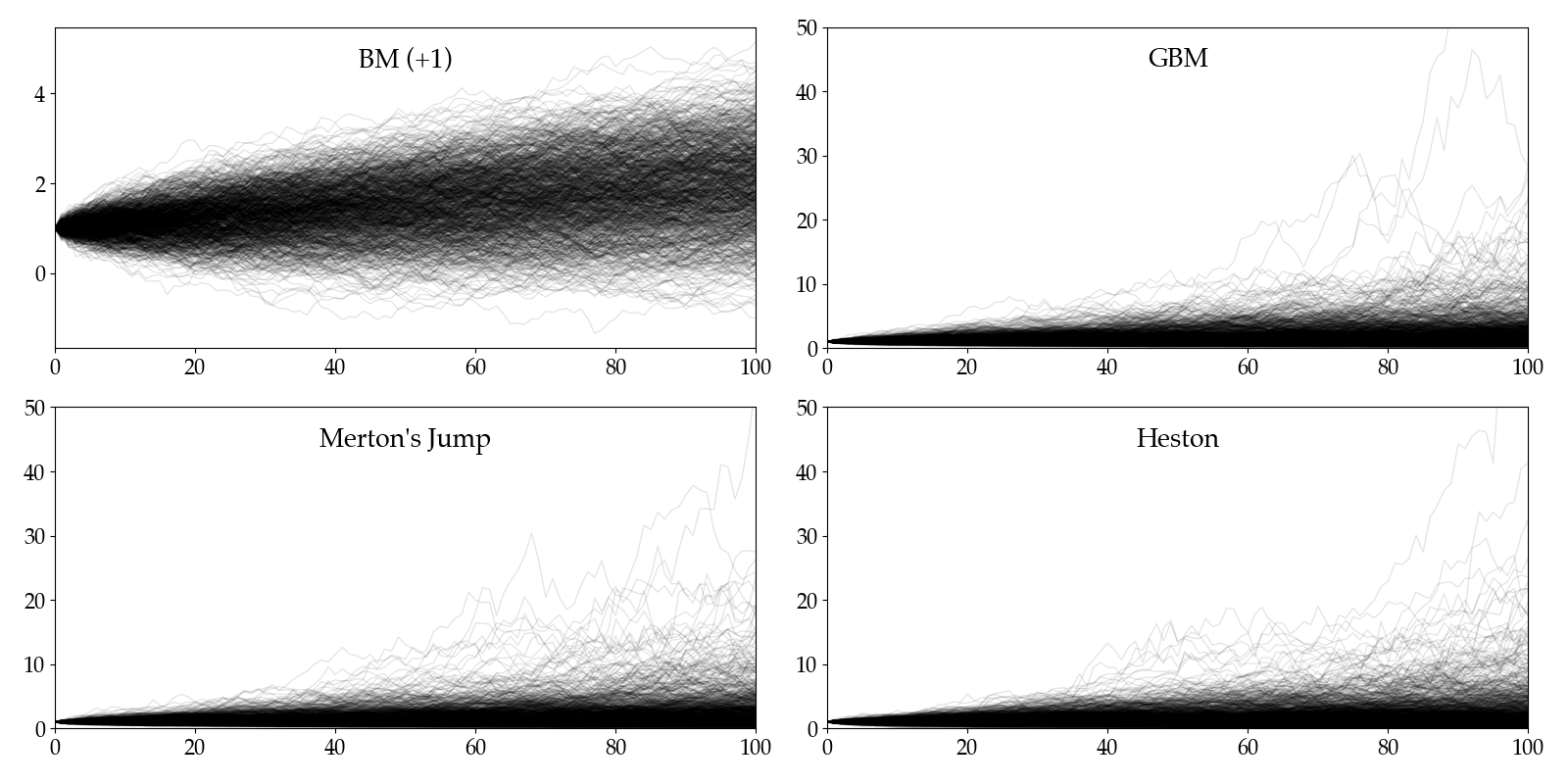
Plots
Finally, let’s take a look at all the simulated price processes. The Brownian motion is shifted s.t. $S_0=1$ like the rest models. Mutual parameters like $\mu$ and $\sigma$ are set to the same values. Each figure shows $1000$ paths.

