I am recently playing a billiard game where you can play a series of exciting tournaments. In each tournament, you pay an entrance fee of, for example, 500USD, to potentially win a prize of, say, 2500USD. There are various kinds of tournaments with different entrance fees ranging from 100USD up to over 10000USD. After hundreds of games, my winning rate stablized around 58%, which is actually pretty good as it significantly beats random draws. A natural concept therefore came into my mind: Is there an optimal strategy?

Well, I think so. I’ll list two strategies below and try to explore any potential optimality. We can reasonably model these tournaments as repetitive betting with certain fixed physical probability $p$ of winning and odds¹ of $(d-1)$:$1$ against ourselves. Given that there are sufficiently sparse tournament entrance fees, we may model these fees as a real variable $x\in\mathbb{R}_+$ to maximize our long run profitability. Without loss of generality, let’s assume an initial balance of $M_0=0$ and that money in this world is infinitely divisible. The problem then becomes determination of the optimal $x\in[0,1]$ s.t. the expected return is maximized. Nonetheless, regarding different interpretations of this problem we have several solutions. Some are intriguing while others may be frustrating.

Martingale

Let’s first take a look at potential values of $x$ and the corresponding balance trajectories $M_t$. For any $0 \le x \le 1$, we have probability $p$ to get an $x$-fraction of our whole balance $D$-folded and $1-p$ to lose it, that is

$$ \text{E}(M_{t+1}\mid\mathcal{F}_t) = (1-x)M_t + p\cdot xdM_t + (1-p)\cdot 0 = [1 + (pd-1)x] M_t $$

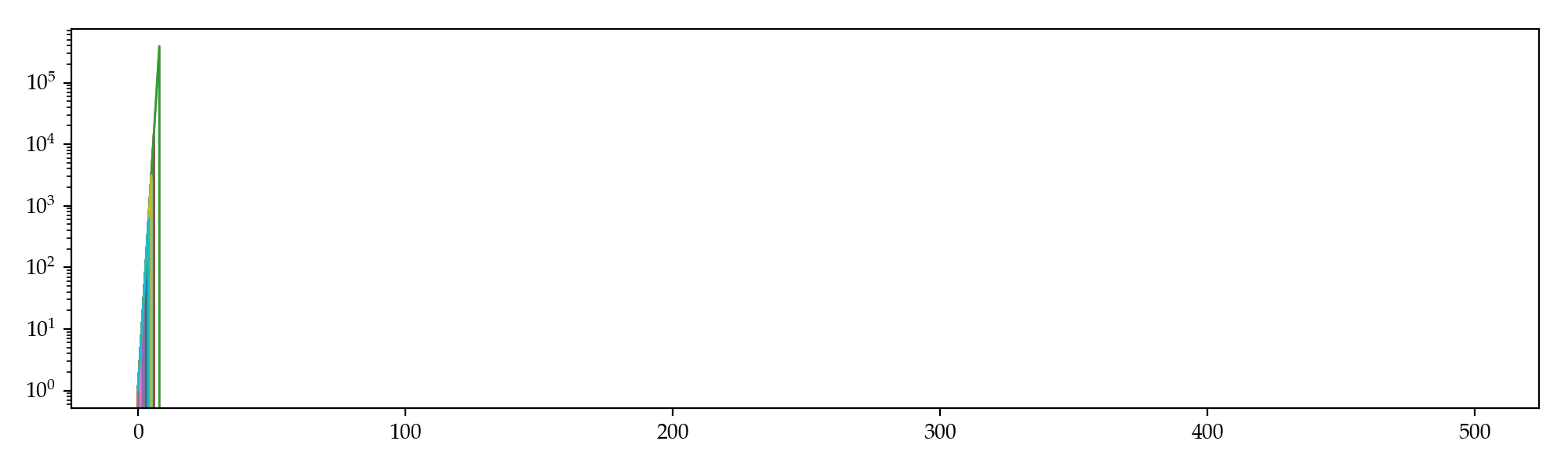
which indicates $M_t$ is a sub-martingale² as in this particular case, $p=0.58$, $d=5$ and thus $pd=2.9 > 1$. So the optimal fraction is $x^* = 1$, which is rather aggresive and yields a ruin probability of $1-p^n$ for the first $n$ bets. Simulation supports our worries: not once did we survived $10$ bets in this tournament, and the maximum we ever attained is less than a million.

Kelly Criterion

If consider $\log M_t$ instead, then

The first order condition is

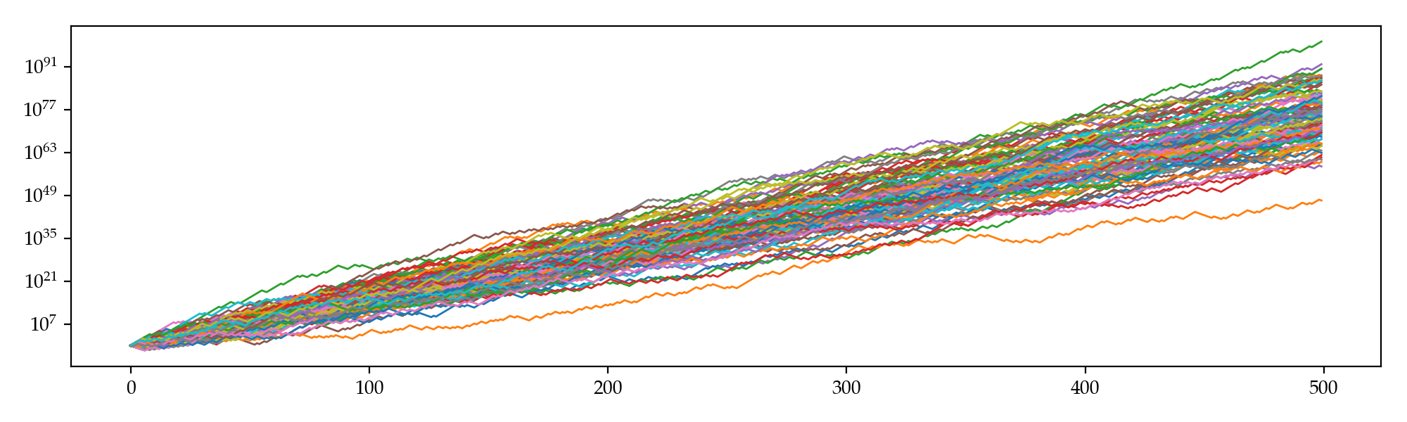
which is more conservative and therefore, should survive longer than the previous strategy. Simulation gives the following trajectories: even the worst sim beat the best we got when $x=1$.

Further Thoughts

According to Doob’s martingale inequality³, the probability of our balance ever attaining a value no less than $C = 1\times10^{60}$ in $T=500$ steps is

$$ \begin{align} &\text{P}\left(\sup_{t \le T}M_t\ge C\right) \le \frac{\text{E}(M_T)}{C} = \frac{M_0}{C} \prod_{t=0}^{T-1}\frac{\text{E}(M_{t+1}\mid\mathcal{F}_t)}{M_t} \&= \frac{[1+(pd-1)x]^T}{C} \approx 4.6\times10^{139} \gg 1. \end{align} $$

This implies the superior limit of the probability that our balance exceeds $1\times10^{60}$ within $500$ steps is one (instead of what simulation gave us, which is around $0.31$). To put it differently, we actually might be able to find a certain strategy that is even significantly better than the one given by the Kelly criterion.

What is it, then? Or, does it actually exist? I don’t have an idea yet, but perhaps exploratory algorithms like machine learning will give us some hints, and perhaps the strategy is not static but rather dynamic.