Basic Walkthrough of ARMA: Take AAPL for Example
2017-03-11
The ARMA model consists of two parts: Auto-Regressive and Moving Average. This is a powerful tool in predicting stationary time series. Today, we’re going to apply it on the stock price of Apple Inc. We will perform the prediction mainly in four parts:
- Data loading
- Decomposition
- ARMA: fit and predict
- Evaluation
After the whole process, there’re some TBD concerns.
Data loading
import pandas as pd
import numpy as np
import matplotlib.pyplot as plt
from yahoo_finance import Share
from datetime import datetime
from statsmodels.tsa.seasonal import seasonal_decompose
from statsmodels.tsa.stattools import adfuller, acf, pacf, arma_order_select_ic
from statsmodels.tsa.arima_model import ARMA, _arma_predict_out_of_sample
np.random.seed(123)    # fix random seed for reproducibility
pd.set_option('display.width', 1000)
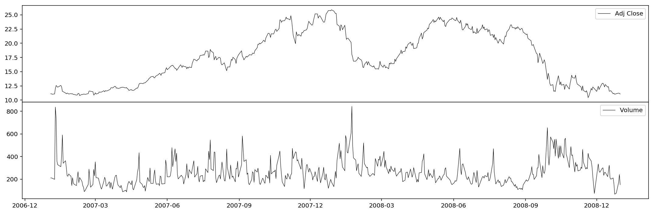
Here we extract the historical data of AAPL from 2007-01-01 to 2009-01-01, which exactly covers the explosion of 2008 subprime crisis. We only consider adjusted close prices and volumes.
# load the dataset
start = '2007-01-01'
end = '2009-01-01'
AAPL = Share('AAPL')
historical = AAPL.get_historical(start_date=start, end_date=end)
df = pd.DataFrame(historical).ix[::-1,['Date','Adj_Close','Volume']]
df = df.set_index('Date').astype(np.float64)
df.index = pd.to_datetime(df.index)
df.Volume /= 1e6  # volume in millions
df.ix[0,:] = df.ix[1,:]
print(df.tail())
print(df.dtypes)
            Adj_Close    Volume
Date
2008-12-24  11.017744   67.8335
2008-12-26  11.117505   77.0812
2008-12-29  11.221153  171.5000
2008-12-30  11.179694  241.9004
2008-12-31  11.057907  151.8853
Adj_Close    float64
Volume       float64
dtype: object
As you can see, I here devide the volume by some properly large number so that the scales of the variables are similar.
print(df.describe())
        Adj_Close      Volume
count  504.000000  504.000000
mean    17.510924  264.179629
std      4.551519  111.138634
min     10.428248   67.833500
25%     12.748336  188.703025
50%     17.160162  240.869300
75%     21.891029  308.259350
max     25.889884  843.242400
%config InlineBackend.figure_format = 'retina'
plt.figure(figsize=(15,5))

ax1 = plt.subplot2grid((2,1), (0,0))
ax1.plot(df.Adj_Close, lw=0.6, color='k')
ax1.set_xlabel('')
ax1.get_xaxis().set_visible(False)
ax1.legend(['Adj Close'])

ax2 = plt.subplot2grid((2,1), (1,0))
ax2.plot(df.Volume, lw=0.6, color='k')
ax2.legend(['Volume'])

plt.tight_layout()
plt.subplots_adjust(hspace=0)
plt.show()
Decomposition
First we take the logarithm of the series. This is totally reversible and in many cases w.r.t. time series could efficiently improve the stationarity.
df = np.log(df)
Then we decompose the series by three parts: trend, seasonality and residual.
dec_Adj_Close = seasonal_decompose(df.Adj_Close, model='multiplicative', freq=60)
dec_Volume = seasonal_decompose(df.Volume, model='multiplicative', freq=60)
The charts are plotted below.
%config InlineBackend.figure_format = 'retina'
plt.figure(figsize=(15,10))

ax1 = plt.subplot2grid((4,2), (0,0))
ax1.plot(df.Adj_Close, lw=0.6, color='k')
ax1.get_xaxis().set_visible(False)
ax1.legend(['original'], loc='upper right')
ax1.set_title('Adj Close')

ax2 = plt.subplot2grid((4,2), (1,0))
ax2.plot(dec_Adj_Close.trend, lw=0.6,  color='k')
ax2.get_xaxis().set_visible(False)
ax2.legend(['trend'], loc='upper right')

ax3 = plt.subplot2grid((4,2), (2,0))
ax3.plot(dec_Adj_Close.seasonal, lw=0.6,  color='k')
ax3.get_xaxis().set_visible(False)
ax3.legend(['seasonality'], loc='upper right')

ax4 = plt.subplot2grid((4,2), (3,0))
ax4.plot(dec_Adj_Close.resid, lw=0.6,  color='k')
ax4.legend(['residual'], loc='upper right')

ax5 = plt.subplot2grid((4,2), (0,1))
ax5.plot(df.Volume, lw=0.6, color='k')
ax5.get_xaxis().set_visible(False)
ax5.legend(['original'], loc='upper right')
ax5.set_title('Volume')

ax6 = plt.subplot2grid((4,2), (1,1))
ax6.plot(dec_Volume.trend, lw=0.6,  color='k')
ax6.get_xaxis().set_visible(False)
ax6.legend(['trend'], loc='upper right')

ax7 = plt.subplot2grid((4,2), (2,1))
ax7.plot(dec_Volume.seasonal, lw=0.6,  color='k')
ax7.get_xaxis().set_visible(False)
ax7.legend(['seasonality'], loc='upper right')

ax8 = plt.subplot2grid((4,2), (3,1))
ax8.plot(dec_Volume.resid, lw=0.6,  color='k')
ax8.legend(['residual'], loc='upper right')

plt.tight_layout()
plt.subplots_adjust(hspace=0)

plt.show()
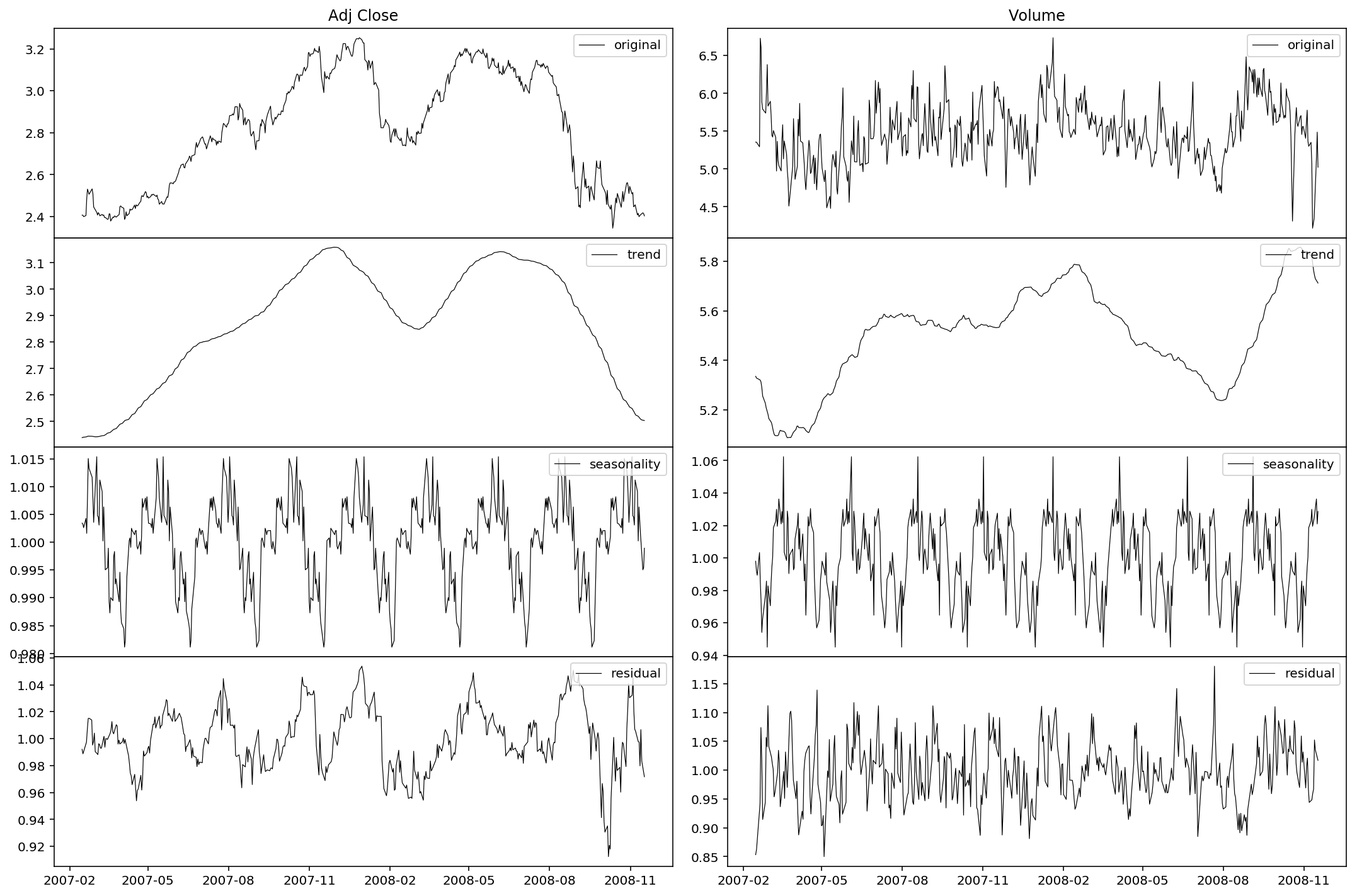
As we can see, the seasonality is periodically significant. Also we may notice the trend behavior in late 2008: a continuous slump in the price and a lagged surge in the volume. The market panic is well illustrated. It’s sure that the seasonality is stationary, but as for the residual, it remains to be tested. Now let’s define a function to test the stationarity of the residuals. We use the Dickey-Fuller test to examine the existence of a unit root.
%config InlineBackend.figure_format = 'retina'
def test_stationarity(timeseries):
    #Determing rolling statistics
    rolmean = timeseries.rolling(center=False, window=12).mean()
    rolstd = timeseries.rolling(center=False, window=12).std()

    #Plot rolling statistics:
    plt.figure(figsize=(15,5))
    orig = plt.plot(timeseries, 'k-', lw=0.6, label='Original')
    mean = plt.plot(rolmean, 'k:', lw=0.6, label='Rolling Mean')
    std = plt.plot(rolstd, 'k-', alpha=0.2, lw=0.6, label = 'Rolling Std')
    plt.legend()
    plt.title('Rolling Mean & Standard Deviation')
    plt.tight_layout()
    plt.show()

    #Perform Dickey-Fuller test:
    print('Results of Dickey-Fuller Test:')
    dftest = adfuller(timeseries, autolag='AIC')
    dfoutput = pd.Series(dftest[0:4], index=['Test Statistic','p-value','#Lags Used','Number of Observations Used'])
    for key,value in dftest[4].items():
        dfoutput['Critical Value (%s)'%key] = value
    print(dfoutput)
Now let’s use our test function.
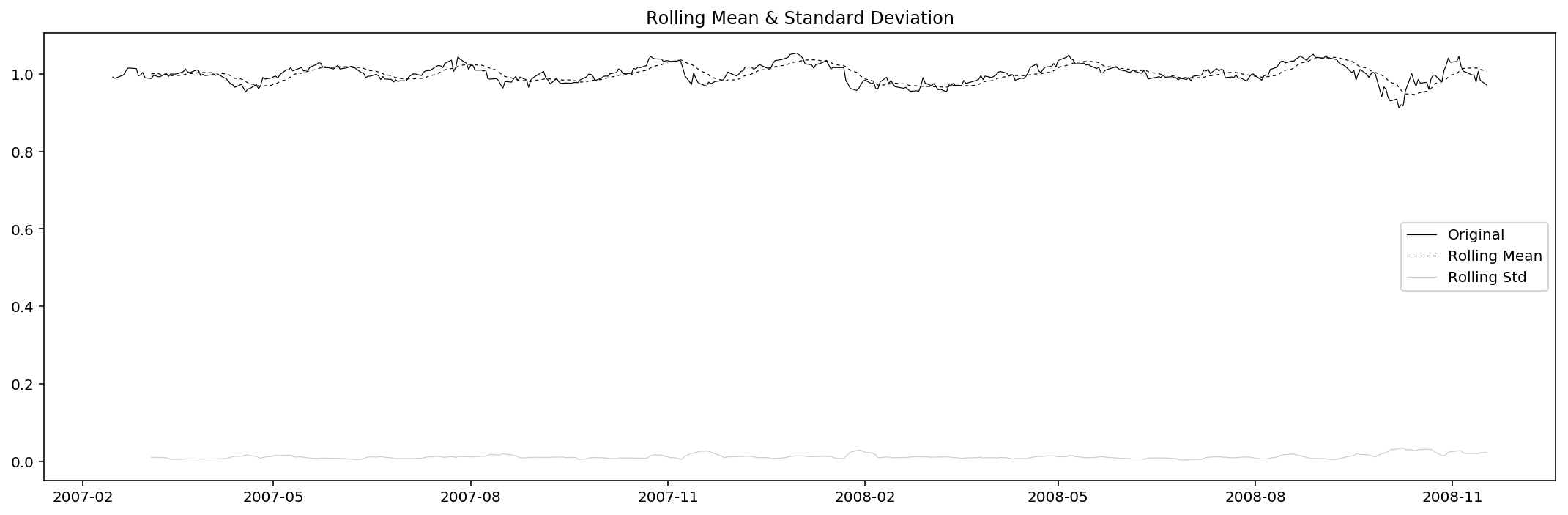
res_Adj_Close = dec_Adj_Close.resid.dropna()
test_stationarity(res_Adj_Close)
Results of Dickey-Fuller Test:
Test Statistic                -5.663466e+00
p-value                        9.265660e-07
#Lags Used                     1.600000e+01
Number of Observations Used    4.270000e+02
Critical Value (1%)           -3.445758e+00
Critical Value (5%)           -2.868333e+00
Critical Value (10%)          -2.570388e+00
dtype: float64
Since the test tatistic is way smaller than the 1% critical value (and the p-value also really small), we reject the null, i.e. we take it that the residual of adjusted close price is stationary under 1% significance level.
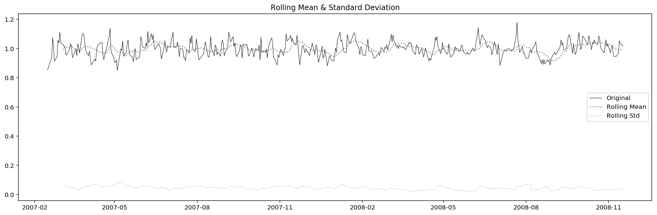
res_Volume = dec_Volume.resid.dropna()
test_stationarity(res_Volume)
Results of Dickey-Fuller Test:
Test Statistic                -1.165042e+01
p-value                        2.043672e-21
#Lags Used                     0.000000e+00
Number of Observations Used    4.430000e+02
Critical Value (1%)           -3.445198e+00
Critical Value (5%)           -2.868086e+00
Critical Value (10%)          -2.570257e+00
dtype: float64
Similar to that of adjusted close price, the residual of volume is considered to be stationary under 1% significance level.
ARMA: fit and predict
Now with stationary time series, we can start forecasting. There are two situations:
- A strictly stationary series with no dependence on past values.
- A series with significant dependence on past values. In this case we need to use some statistical models like ARMA to forecast the data.
Here we are of course using the latter one, and thus we need to specify the parameters of the model:
- Number of AR (Auto-Regressive) terms (
$p$): AR terms are just lags of dependent variable. For instance if$p$is$5$, the predictors for$x_t$will be$x_{t-1},x_{t-2},\ldots,x_{t-5}$. - Number of MA (Moving Average) terms (
$q$): MA terms are lagged forecast errors in prediction equation. For instance if$q$is$5$, the predictors for$x_t$will be$e_{t-1},e_{t-2},\ldots,e_{t-5}$where$e_i$is the difference between the moving average at$i^{th}$instant and actual value.
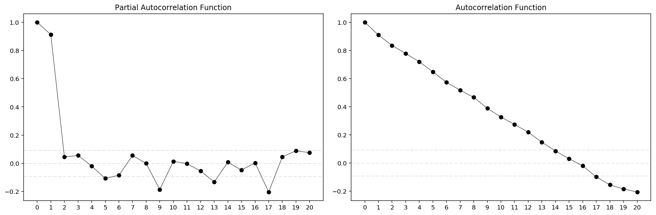
An importance concern here is how to determine the values of $p$ and $q$. Below we plot the ACF and PACF charts to determine them. The rules are:
$p$: The lag value where the PACF chart crosses the upper confidence interval for the first time.$q$: The lag value where the ACF chart crosses the upper confidence interval for the first time.
So first, let’s plot the ACF and PACF charts.
%config InlineBackend.figure_format = 'retina'
def acfplot(timeseries):
    #ACF and PACF plots:
    nlags = 20

    #Pre-set ACF and PACF:
    lag_acf = acf(timeseries, nlags=nlags)
    lag_pacf = pacf(timeseries, nlags=nlags, method='ols')

    fig = plt.figure(figsize=(15,5))

    #Plot PACF:
    ax1 = fig.add_subplot(121)
    ax1.plot(lag_pacf, 'ko-', lw=0.6)
    ax1.set_xticks(range(nlags+1))
    ax1.axhline(y=0, ls='--', c='k', lw=0.6, alpha=0.2)
    ax1.axhline(y=-1.96/np.sqrt(len(timeseries)), ls='--', c='k', lw=0.6, alpha=0.2)
    ax1.axhline(y=1.96/np.sqrt(len(timeseries)), ls='--', c='k', lw=0.6, alpha=0.2)
    ax1.set_title('Partial Autocorrelation Function')

    #Plot ACF:
    ax2 = fig.add_subplot(122)
    ax2.plot(lag_acf, 'ko-', lw=0.6)
    ax2.set_xticks(range(nlags+1))
    ax2.axhline(y=0, ls='--', c='k', lw=0.6, alpha=0.2)
    ax2.axhline(y=-1.96/np.sqrt(len(timeseries)), ls='--', c='k', lw=0.6, alpha=0.2)
    ax2.axhline(y=1.96/np.sqrt(len(timeseries)), ls='--', c='k', lw=0.6, alpha=0.2)
    ax2.set_title('Autocorrelation Function')

    plt.tight_layout()
    plt.show()
acfplot(res_Adj_Close)
acfplot(res_Volume)
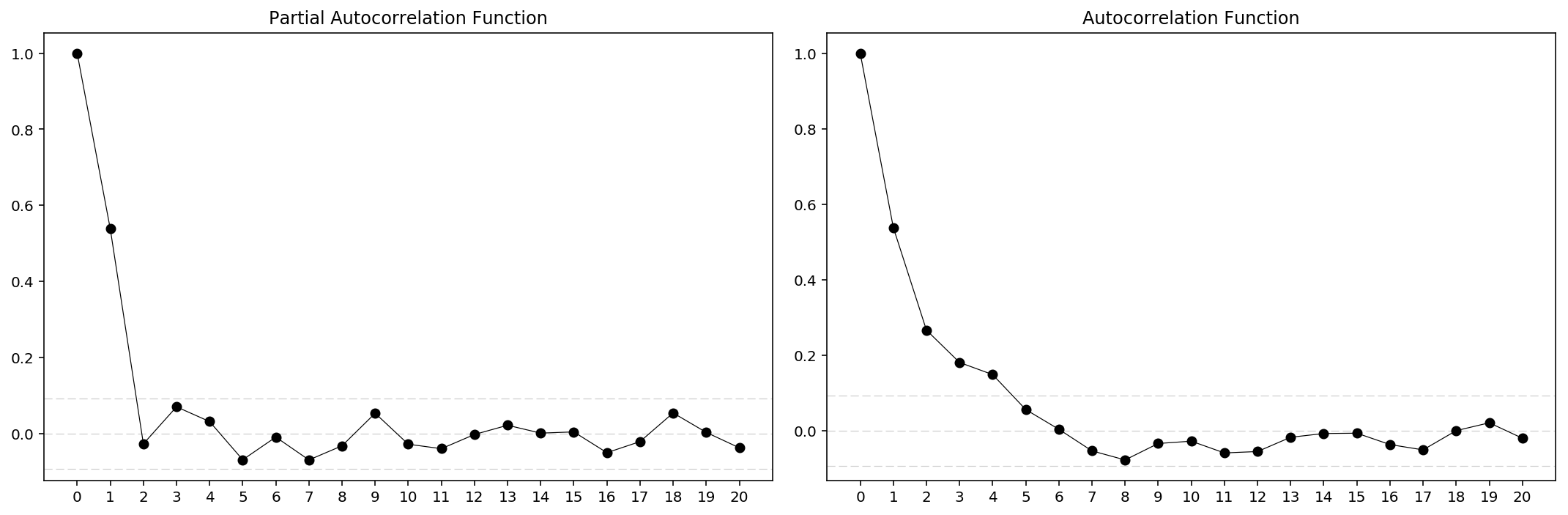
From the charts it is clear that for $Adj\ Close$ we have $p=2$, $q=14$ and for $Volume$ we have $p=2$, $q=5$. Then we can load the ARIMA models for prediction. However, there’re actually built-in method for that, which is quite more direct.
order = arma_order_select_ic(res_Adj_Close, max_ar=5, max_ma=20, ic=['aic', 'bic', 'hqic'])
order.bic_min_order
/Users/Allen_Frostline/anaconda3/lib/python3.6/site-packages/statsmodels/base/model.py:466: ConvergenceWarning: Maximum Likelihood optimization failed to converge. Check mle_retvals
  "Check mle_retvals", ConvergenceWarning)
/Users/Allen_Frostline/anaconda3/lib/python3.6/site-packages/statsmodels/base/model.py:466: ConvergenceWarning: Maximum Likelihood optimization failed to converge. Check mle_retvals
  "Check mle_retvals", ConvergenceWarning)
...
/Users/Allen_Frostline/anaconda3/lib/python3.6/site-packages/statsmodels/base/model.py:466: ConvergenceWarning: Maximum Likelihood optimization failed to converge. Check mle_retvals
  "Check mle_retvals", ConvergenceWarning)


(1, 0)
… and yes, unreliable and horribly slow. Just forget about that. Let’s continue with the ARMA model.
%config InlineBackend.figure_format = 'retina'
def pred(timeseries, p, q):
    model = ARMA(timeseries, (p, q)).fit()
    pred = model.fittedvalues
    plt.close()
    plt.figure(figsize=(15,5))
    plt.plot(timeseries, 'k-', lw=0.6, label='true data')
    plt.plot(pred, 'k:', lw=0.6, label='prediction')
    plt.title('$R_{{adj}}^2$ : {:.4f}'.format(1-(sum((pred - timeseries)**2)/(len(timeseries)-p-q-1))/(sum(timeseries**2)/(len(timeseries)-1)))) # Residual Sum of Squares, RSS = SUM[(y-f(x))^2]
    plt.legend(loc='upper right')
    plt.tight_layout()
    plt.show()
    return model, pred
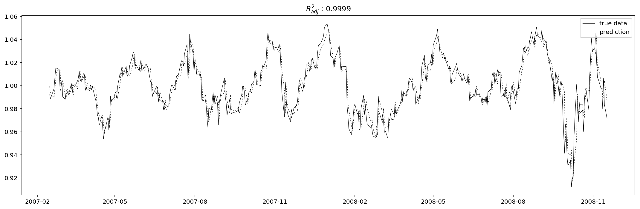
model_res_Adj_Close, pred_res_Adj_Close = pred(res_Adj_Close, 2, 14)
/Users/Allen_Frostline/anaconda3/lib/python3.6/site-packages/statsmodels/base/model.py:466: ConvergenceWarning: Maximum Likelihood optimization failed to converge. Check mle_retvals
  "Check mle_retvals", ConvergenceWarning)
model_res_Volume, pred_res_Volume = pred(res_Volume, 2, 5)
/Users/Allen_Frostline/anaconda3/lib/python3.6/site-packages/statsmodels/base/model.py:466: ConvergenceWarning: Maximum Likelihood optimization failed to converge. Check mle_retvals
  "Check mle_retvals", ConvergenceWarning)
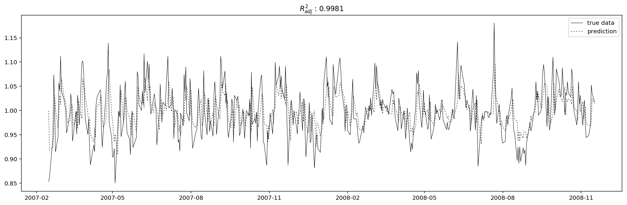
Evaluation
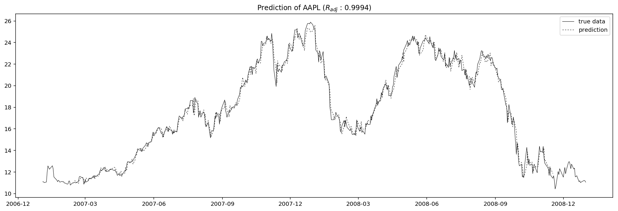
Just as what I did above, I use adjusted R-square as the evaluation metric function. The “adjusted” means the R-square is punished for too many explanatory variables, and thus can in a way reduce the tendency of overfitting.
%config InlineBackend.figure_format = 'retina'
plt.figure(figsize=(15,5))
pred = dec_Adj_Close.trend * dec_Adj_Close.seasonal * pred_res_Adj_Close
data = np.exp(df.Adj_Close)
pred = np.exp(pred)
plt.plot(data, 'k-', lw=0.6, label='true data')
plt.plot(pred, 'k:', lw=0.6, label='prediction')
plt.tight_layout()
plt.legend()
plt.title('Prediction of AAPL ($R_{{adj}}$ : {:.4f})'.format(1-(sum((pred - data).dropna()**2)/(len(data)-2-14-1))/(sum(data.dropna()**2)/(len(data)-1))))
plt.show()
%config InlineBackend.figure_format = 'retina'
plt.figure(figsize=(15,5))
pred = dec_Volume.trend * dec_Volume.seasonal * pred_res_Volume
data = np.exp(df.Volume) * 1e6
pred = np.exp(pred) * 1e6
plt.plot(data, 'k-', lw=0.6, label='true data')
plt.plot(pred, 'k:', lw=0.6, label='prediction')
plt.tight_layout()
plt.legend()
plt.title('Prediction of AAPL ($R_{{adj}}$ : {:.4f})'.format(1-(sum((pred - data).dropna()**2)/(len(data)-2-5-1))/(sum(data.dropna()**2)/(len(data)-1))))
plt.show()
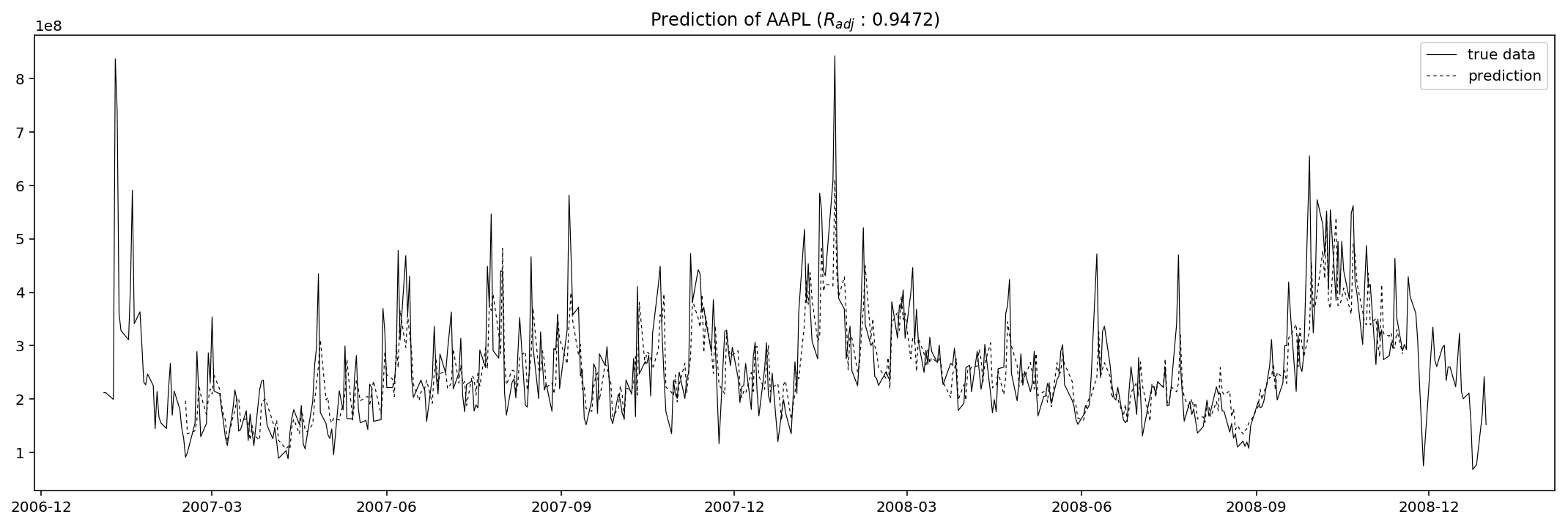
The results seem good, but never forget that this is only the in-sample prediction, so in other words this could be totally an opposite scenario when we use this fitted model to predict out-sample values, i.e. to predict the adjusted close or volume on 2009-01-02 (a Friday).
params = model_res_Adj_Close.params
residuals = model_res_Adj_Close.resid
p = model_res_Adj_Close.k_ar
q = model_res_Adj_Close.k_ma
k_exog = model_res_Adj_Close.k_exog
k_trend = model_res_Adj_Close.k_trend
steps = 5

_arma_predict_out_of_sample(params, steps, residuals, p, q, k_trend, k_exog, endog=res_Adj_Close, exog=None, start=len(res_Adj_Close)).squeeze()
array([ 0.97023813, 0.97742186, 0.97331353, 0.97333901, 0.981861 ])
params = model_res_Volume.params
residuals = model_res_Volume.resid
p = model_res_Volume.k_ar
q = model_res_Volume.k_ma
k_exog = model_res_Volume.k_exog
k_trend = model_res_Volume.k_trend
steps = 5

_arma_predict_out_of_sample(params, steps, residuals, p, q, k_trend, k_exog, endog=res_Volume, exog=None, start=len(res_Volume)).squeeze()
array([ 1.00925408, 1.01171945, 1.00450219, 0.99949544, 0.99683326])
Conclusion & concerns
Another concern is (which is really obvious), that here when back-computing the predicted values I used the formular
$$ Y_{total} = Y_{trend} \cdot Y_{seasonality} \cdot Y_{residual} $$
but only the residual is predicted using our ARMA model. The rest two parts, of cource, should also be predicted and then we can finally call it a “prediction”. Otherwise we are only partially predicting the series. For the seasonality we may directly do a translation as the patterns are very stable. However, as for the trend composition, neither translation nor ARMA are going to work well. My suggestion is to resort to deep learning or some RNN models (like LSTM in another post of mine). Machine learning in the field of time series prediction is indeed promising and stunning in recent years.
Another concern, which is actually way more important, is that we lack out-sample prediction here. This is also called cross validation. Why is cross validation so important? Because if we don’t do any cross validation, then we can always use as many explanatory variables as possible to achieve better scores in evaluation, which is most likely how overfitting happens. What we are gonna do to eliminate this, is to use historical data within time range, say, from 2009-01-01 to 2009-06-01, to predict the adjusted close prices and volumes day by day. The adjusted R-square is then the “test score” of the model, while implicitly the former R-square becomes the “train score”.
References:
- McKinney, Wes, Josef Perktold, and Skipper Seabold. “Time series analysis in Python with statsmodels.” Jarrodmillman. Com (2011): 96-102.
- Kwiatkowski, Denis, et al. “Testing the null hypothesis of stationarity against the alternative of a unit root: How sure are we that economic time series have a unit root?.” Journal of econometrics 54.1-3 (1992): 159-178.
- 竹间为简, “AR(I)MA时间序列建模过程”.
- Seasonal ARIMA with Python
- 有什么好的模型可以做高精度的时间序列预测呢?
- Machine Learning Strategies for Time Series Prediction
- A Youtube Course on AR, MA, ARMA and ARIMA