Bitcoin Inter-exchange Price Spread Prediction
2017-05-21
Price prediction is thought to be very difficult for any equity, however the price spread between two exchanges may not. We look into the price spread between two of the largest Bitcoin exchanges: Bitstamp and BTC-E.
Step 1: Import All Packages
import quandl
import cmocean
import warnings
import numpy as np
import pandas as pd
import seaborn as sns
import statsmodels.api as sm
from pytrends.request import TrendReq
from scipy import stats as ss
from datetime import datetime as dt
from arch.unitroot import PhillipsPerron, ADF
from matplotlib import pyplot as plt
from matplotlib import dates as mdates
from statsmodels.graphics.api import qqplot
pytrend = TrendReq('[email protected]', 'aaaaaaaaaa', hl='en-US', tz=360, custom_useragent=None)
warnings.filterwarnings('ignore')
quandl.ApiConfig.api_key = 'aaaaaaaaaaaaaaa'
pd.set_option("display.width",999)
plt.rcdefaults()
plt.style.use('seaborn-paper')
plt.rcParams['axes.facecolor']='w'
plt.rcParams['axes.grid']=False
plt.rcParams['font.family'] = 'serif'
plt.rcParams['figure.figsize'] = [12, 4]
Step 2: Data Retrieving and Cleaning
Data source: https://www.quandl.com/data/.
exchangelist = [
    'BTCE',
    'KRAKEN',
    'BITFINEX',
    'BITSTAMP',
#     'COINBASE',
    'ROCK',
    'HITBTC',
    'ITBIT',
    'BITBAY',
    'BITKONAN',
    'CBX',
    'VCX'
]
n = len(exchangelist)
print('there are {} exchanges in total'.format(n))
there are 11 exchanges in total
exchanges = [quandl.get('BCHARTS/' + e + 'USD') for e in exchangelist]
for i in range(n):
    daterange = exchanges[i].index.tolist()
    print('{:>8}'.format(exchangelist[i]), daterange[0].date(), daterange[-1].date())
    BTCE 2011-08-14 2017-05-19
  KRAKEN 2014-01-07 2017-05-19
BITFINEX 2013-03-31 2016-12-22
BITSTAMP 2011-09-13 2017-05-19
    ROCK 2011-11-12 2017-05-19
  HITBTC 2013-12-27 2017-05-19
   ITBIT 2013-08-25 2017-05-19
  BITBAY 2014-05-16 2017-05-19
BITKONAN 2013-07-02 2017-05-19
     CBX 2011-07-05 2017-04-16
     VCX 2011-12-25 2017-05-19
start_date = pd.to_datetime('2014-07-01')
mid_date = pd.to_datetime('2016-01-01')
end_date = pd.to_datetime('2016-07-01')
price = pd.concat([e.ix[start_date:end_date,'Close'] for e in exchanges], join='outer', axis=1)
volume = pd.concat([e.ix[start_date:end_date,'Volume (Currency)'] for e in exchanges], join='outer', axis=1)
price.columns = exchangelist
volume.columns = exchangelist
price = price[price > 0].fillna(method='ffill').fillna(method='bfill')
volume = price[volume > 0].fillna(method='ffill').fillna(method='bfill')
print(price.describe())
             BTCE      KRAKEN    BITFINEX    BITSTAMP        ROCK      HITBTC       ITBIT      BITBAY    BITKONAN         CBX         VCX
count  732.000000  732.000000  732.000000  732.000000  732.000000  732.000000  732.000000  732.000000  732.000000  732.000000  732.000000
mean   359.045682  363.799398  363.647027  363.204795  363.963907  373.581913  362.888860  367.052036  369.847240  367.836366  388.325161
std    119.611681  122.473245  122.182031  122.020091  121.643524  115.354405  121.729241  125.084653  123.984738  119.057448   94.745641
min    170.000000  175.000000  182.000000  171.410000  185.000000  186.760000  183.160000  186.890000  171.030000  200.040000  210.000001
25%    245.123250  249.669390  249.235000  249.047500  249.887500  272.900000  249.252500  253.750000  254.972500  254.757500  312.249915
50%    349.933000  358.429990  353.825000  356.495000  355.015000  357.610000  353.475000  359.995000  360.765000  365.005000  380.000000
75%    429.812500  430.136262  433.410000  432.535000  433.282500  438.695000  432.302500  435.082500  442.192500  432.992500  425.000000
max    729.855000  765.490000  769.500000  766.620000  767.800000  768.590000  767.180000  999.000000  771.670000  690.000000  658.000000
Step 3: Data Analysis
%config InlineBackend.figure_format = 'retina'
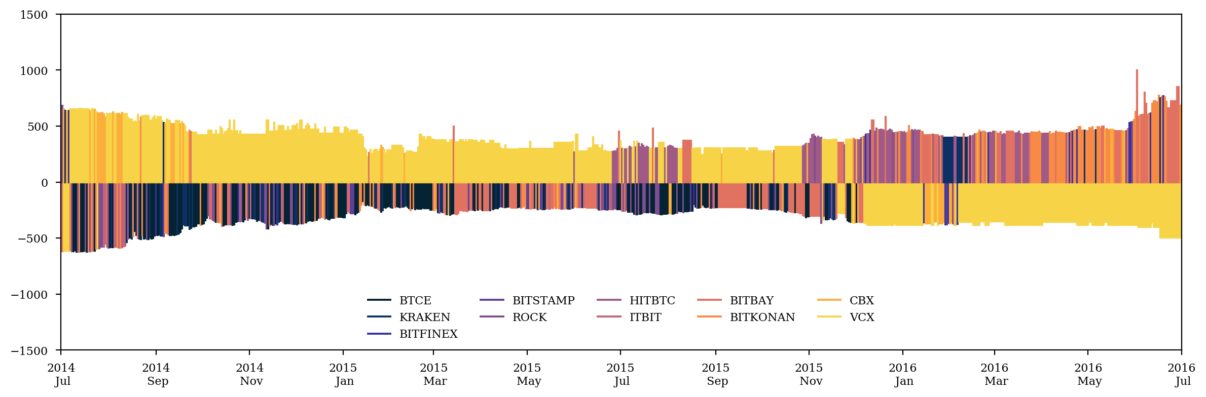
min_exchange = pd.Series([np.argmin(price.iloc[i], axis=0) for i in range(len(price))],
index=price.index).apply(lambda fn: exchangelist.index(fn))
max_exchange = pd.Series([np.argmax(price.iloc[i], axis=0) for i in range(len(price))],
index=price.index).apply(lambda fn: exchangelist.index(fn))
dmin = price.min(axis=1)
dmax = price.max(axis=1)
thermal = cmocean.cm.thermal
plt.close()
fig = plt.figure()
ax = fig.add_subplot(111)
for i in range(n):
ax.plot((price.index[0], price.index[0]), (0, 0), c=thermal(i/n), label=exchangelist[i])
for i in range(len(price)):
ax.plot((price.index[i], price.index[i]), (0, -dmin[i]), lw=1.5, c=thermal(min_exchange[i]/n))
ax.plot((price.index[i], price.index[i]), (0, dmax[i]), lw=1.5, c=thermal(max_exchange[i]/n))
ax.xaxis.set_major_locator(mdates.MonthLocator(interval=2))
ax.xaxis.set_major_formatter(mdates.DateFormatter('%Y\n %b'))
ax.set_xlim(start_date, end_date)
ax.set_ylim(-1500,1500)
plt.legend(loc='lower center', frameon=0, ncol=n//2)
plt.tight_layout()
plt.savefig('price1.pdf')
plt.show()
active_price = price * (price.diff() != 0)
active_price = active_price[active_price > 0]
err_count = np.isnan(active_price).sum()
%config InlineBackend.figure_format = 'retina'
plt.close()
fig = plt.figure()

ax1 = fig.add_subplot(111)
(100*max_exchange.value_counts().sort_index().reindex(range(len(exchangelist))).fillna(0)/len(price)).plot.bar(ax=ax1, color='c', align='center', alpha=.5, label='% being highest')
(100*min_exchange.value_counts().sort_index().reindex(range(len(exchangelist))).fillna(0)/len(price)).plot.bar(ax=ax1, color='r', align='center', alpha=.5, label='% being lowest')
ax1.set_ylim(-5,80)
ax1.set_ylabel('%')
plt.xticks(range(len(err_count)), err_count.index.tolist(), rotation=0)
ax1.legend(loc='upper left', frameon=0)

ax2 = ax1.twinx()
err_count.plot(ax=ax2, marker='o', color='r', alpha=.5, label='total number of error days')
ax2.set_xlim(-.5,len(err_count)-.5)
ax2.set_xticks(range(len(err_count)), err_count.index.tolist())
ax2.legend(loc='upper right', frameon=0)
ax2.set_ylim(-35,500)

# plt.grid(None)
plt.tight_layout()
plt.show()
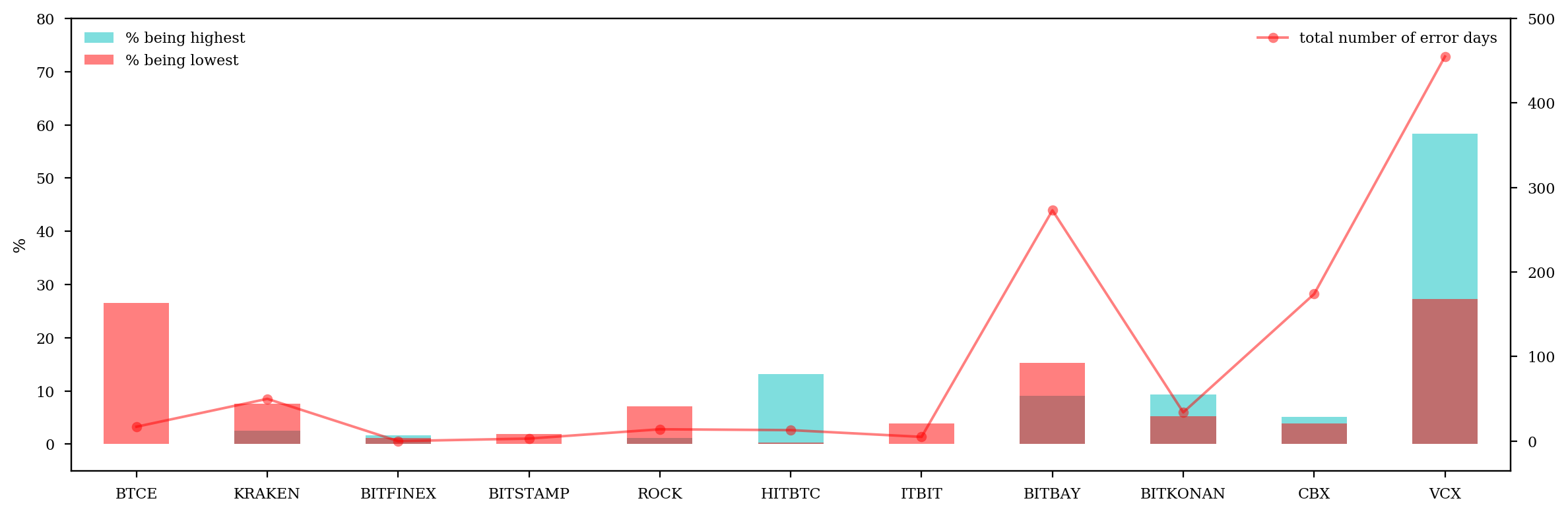
irr_exchanges = [10,9,8,7,5,0]  # delete those that have over 200 error days, or dominate over 10% of all time range
n -= len(irr_exchanges)
active_price.drop(active_price.columns[[irr_exchanges]], axis=1, inplace=1)
for i in irr_exchanges:
    exchangelist.pop(i)
%config InlineBackend.figure_format = 'retina'
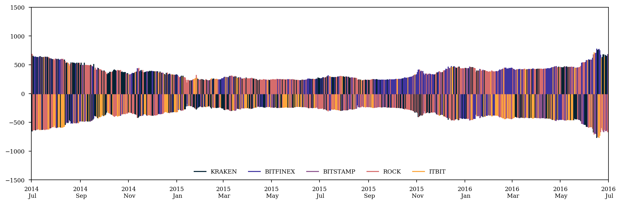
min_exchange = pd.Series([np.argmin(active_price.iloc[i], axis=0) for i in range(len(active_price))], index=active_price.index).apply(lambda fn: exchangelist.index(fn))
dmin = active_price.min(axis=1)
max_exchange = pd.Series([np.argmax(active_price.iloc[i], axis=0) for i in range(len(active_price))], index=active_price.index).apply(lambda fn: exchangelist.index(fn))
dmax = active_price.max(axis=1)
thermal = cmocean.cm.thermal
plt.close()
fig = plt.figure()
ax = fig.add_subplot(111)
for i in range(n):
ax.plot((active_price.index[0], active_price.index[0]), (0, 0), c=thermal(i/n), label=exchangelist[i])
for i in range(len(active_price)):
ax.plot((active_price.index[i], active_price.index[i]), (0, -dmin[i]), lw=1.5, c=thermal(min_exchange[i]/n))
ax.plot((active_price.index[i], active_price.index[i]), (0, dmax[i]), lw=1.5, c=thermal(max_exchange[i]/n))
ax.xaxis.set_major_locator(mdates.MonthLocator(interval=2))
ax.xaxis.set_major_formatter(mdates.DateFormatter('%Y\n %b'))
ax.set_xlim(start_date, end_date)
ax.set_ylim(-1500,1500)
plt.legend(loc='lower center', frameon=0, ncol=n)
plt.tight_layout()
plt.savefig('price2.pdf')
plt.show()
%config InlineBackend.figure_format = 'retina'
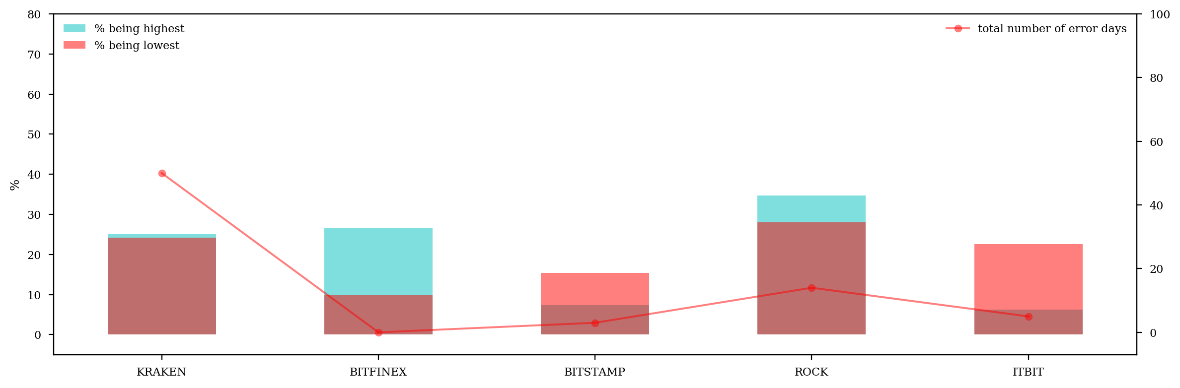
err_count = np.isnan(active_price).sum()
plt.close()
fig = plt.figure()
ax1 = fig.add_subplot(111)
(100*max_exchange.value_counts().sort_index().reindex(range(len(exchangelist))).fillna(0)/len(price)).plot.bar(ax=ax1, color='c', align='center', alpha=.5, label='% being highest')
(100*min_exchange.value_counts().sort_index().reindex(range(len(exchangelist))).fillna(0)/len(price)).plot.bar(ax=ax1, color='r', align='center', alpha=.5, label='% being lowest')
ax1.set_ylim(-5,80)
ax1.set_ylabel('%')
plt.xticks(range(len(err_count)), err_count.index.tolist(), rotation=0)
ax1.legend(loc='upper left', frameon=0)
ax2 = ax1.twinx()
err_count.plot(ax=ax2, marker='o', color='r', alpha=.5, label='total number of error days')
ax2.set_xlim(-.5,len(err_count)-.5)
ax2.set_xticks(range(len(err_count)), err_count.index.tolist())
ax2.legend(loc='upper right', frameon=0)
ax2.set_ylim(-7,100)
# plt.grid(None)
plt.tight_layout()
plt.show()
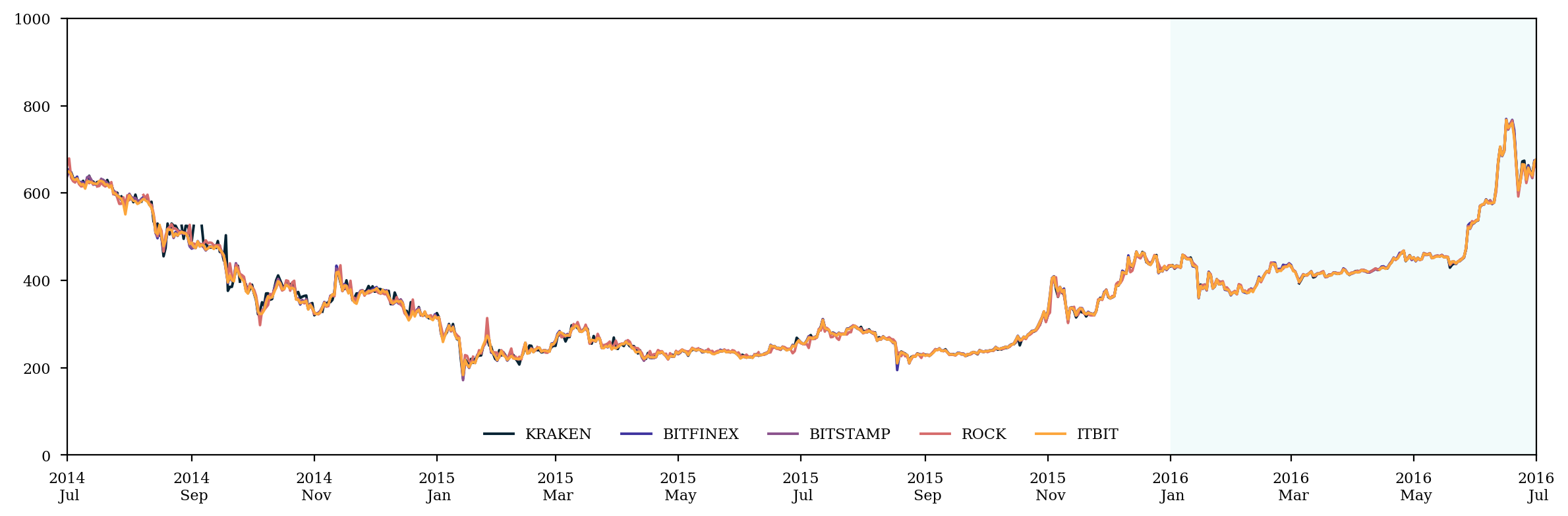
%config InlineBackend.figure_format = 'retina'
plt.close()

fig = plt.figure()

ax = fig.add_subplot(111)
for i in range(n):
    ax.plot(active_price.ix[:,i], c=thermal(i/n), label=exchangelist[i])
ax.xaxis.set_major_locator(mdates.MonthLocator(interval=2))
ax.xaxis.set_major_formatter(mdates.DateFormatter('%Y\n %b'))
ax.axvspan(mid_date, end_date, color='c', alpha=0.05)
ax.set_xlim(start_date, end_date)
ax.set_ylim(0,1000)

plt.legend(loc='lower center', frameon=0, ncol=n)
plt.tight_layout()
# plt.title('Historical Prices')
plt.savefig('price3.pdf')
plt.show()
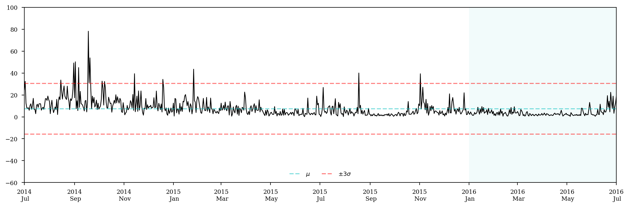
price_spread = active_price.max(axis=1) - active_price.min(axis=1)
price_spread.describe()
count    732.000000
mean       7.418801
std        7.705870
min        0.150000
25%        2.430000
50%        4.914920
75%        9.461703
max       78.191470
dtype: float64
%config InlineBackend.figure_format = 'retina'
plt.close()

fig = plt.figure()

ax = fig.add_subplot(111)
ax.plot(price_spread, lw=1,c='k')
ax.axhline(price_spread.mean(), alpha=0.5, ls='--', c='c', label='$\mu$')
ax.axhline(price_spread.mean()+price_spread.std()*3, alpha=0.5, ls='--', c='r', label='$\pm3\sigma$')
ax.axhline(price_spread.mean()-price_spread.std()*3, alpha=0.5, ls='--', c='r')
ax.xaxis.set_major_locator(mdates.MonthLocator(interval=2))
ax.xaxis.set_major_formatter(mdates.DateFormatter('%Y\n %b'))
ax.axvspan(mid_date, end_date, color='c', alpha=0.05)
ax.set_xlim(start_date, end_date)
ax.set_ylim(-60,100)

plt.tight_layout()
plt.legend(loc='lower center', framealpha=0, ncol=2)
# plt.title('Price Spreads')
plt.savefig('spread.pdf')
plt.show()
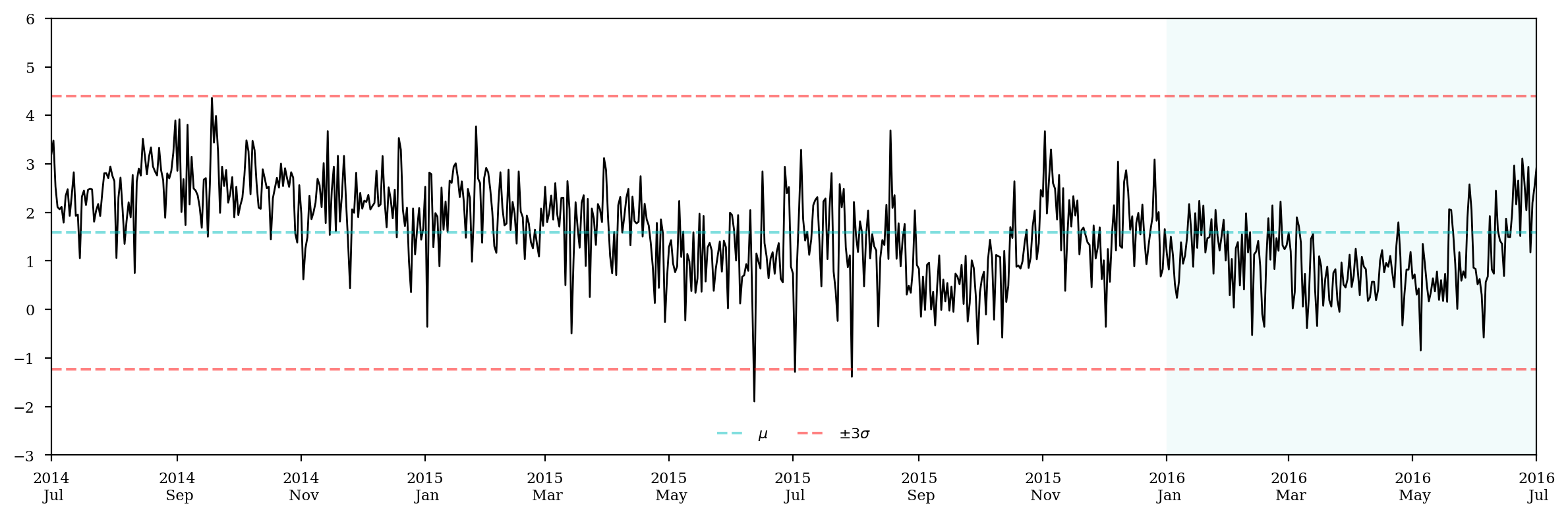
log_price_spread = np.log(price_spread)
log_price_spread.describe()
count    732.000000
mean       1.584788
std        0.939405
min       -1.897120
25%        0.887891
50%        1.592275
75%        2.247244
max        4.359161
dtype: float64
%config InlineBackend.figure_format = 'retina'
plt.close()
fig = plt.figure()
ax = fig.add_subplot(111)
ax.plot(log_price_spread, c='k',lw=1,label='')
ax.axhline(log_price_spread.mean(), alpha=0.5, ls='--', c='c', label='$\mu$')
ax.axhline(log_price_spread.mean()+log_price_spread.std()*3, alpha=0.5, ls='--', c='r',label='$\pm3\sigma$')
ax.axhline(log_price_spread.mean()-log_price_spread.std()*3, alpha=0.5, ls='--', c='r')
ax.xaxis.set_major_locator(mdates.MonthLocator(interval=2))
ax.xaxis.set_major_formatter(mdates.DateFormatter('%Y\n %b'))
ax.axvspan(mid_date, end_date, color='c', alpha=0.05)
ax.set_ylim(-3,6)
ax.set_xlim(start_date, end_date)
plt.tight_layout()
plt.legend(loc='lower center', framealpha=0, ncol=2)
# plt.title('Log Price Spreads')
plt.savefig('logspread.pdf')
plt.show()
print(ADF(log_price_spread, trend='c'), '\n')
print(PhillipsPerron(log_price_spread, trend='c'), '\n')
   Augmented Dickey-Fuller Results
=====================================
Test Statistic                 -2.346
P-value                         0.158
Lags                               17
-------------------------------------

Trend: Constant
Critical Values: -3.44 (1%), -2.87 (5%), -2.57 (10%)
Null Hypothesis: The process contains a unit root.
Alternative Hypothesis: The process is weakly stationary.

     Phillips-Perron Test (Z-tau)
=====================================
Test Statistic                -21.389
P-value                         0.000
Lags                               20
-------------------------------------
Trend: Constant Critical Values: -3.44 (1%), -2.87 (5%), -2.57 (10%) Null Hypothesis: The process contains a unit root. Alternative Hypothesis: The process is weakly stationary.
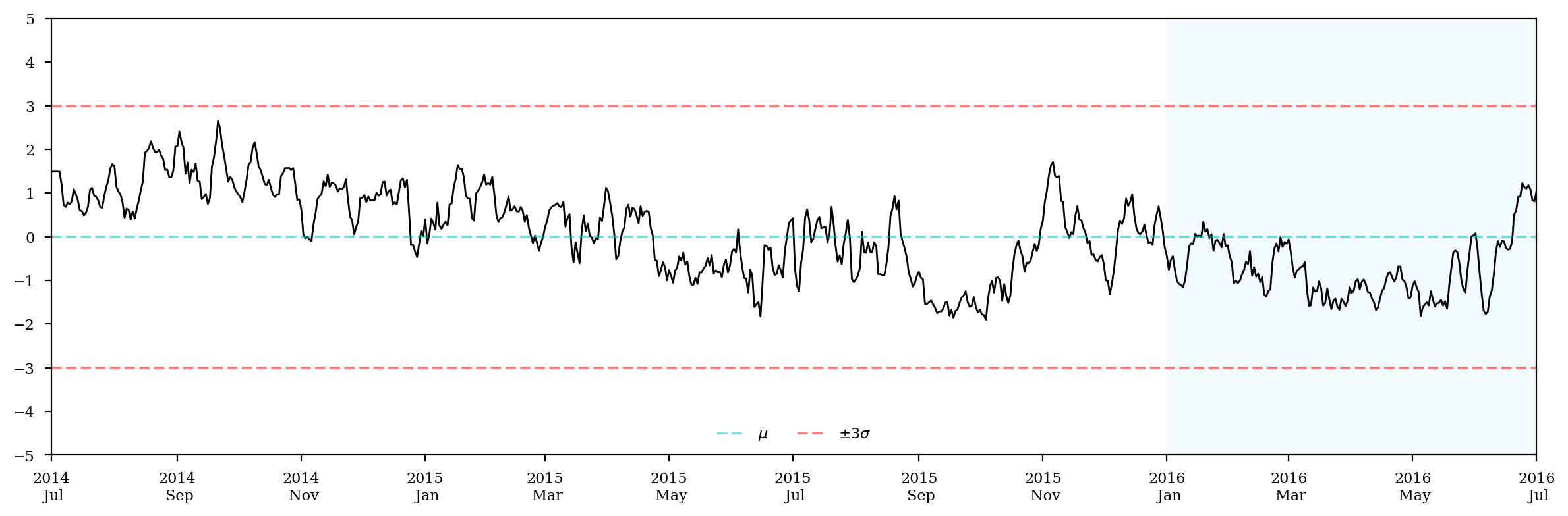
def z_norm(s):
    return (s - s.mean(axis=0)) / s.std(axis=0)
log_price_spread = z_norm(log_price_spread.rolling(5).mean().fillna(method='bfill'))
log_price_spread.describe()
count    7.320000e+02
mean    -4.284976e-15
std      1.000000e+00
min     -1.902323e+00
25%     -8.414662e-01
50%     -1.734537e-02
75%      7.996859e-01
max      2.645812e+00
Name: None, dtype: float64
print(ADF(log_price_spread, trend='nc'), '\n')
print(PhillipsPerron(log_price_spread, trend='nc'), '\n')
   Augmented Dickey-Fuller Results
=====================================
Test Statistic                 -2.229
P-value                         0.025
Lags                               20
-------------------------------------

Trend: No Trend
Critical Values: -2.57 (1%), -1.94 (5%), -1.62 (10%)
Null Hypothesis: The process contains a unit root.
Alternative Hypothesis: The process is weakly stationary.

     Phillips-Perron Test (Z-tau)
=====================================
Test Statistic                 -3.321
P-value                         0.001
Lags                               20
-------------------------------------

Trend: No Trend
Critical Values: -2.57 (1%), -1.94 (5%), -1.62 (10%)
Null Hypothesis: The process contains a unit root.
Alternative Hypothesis: The process is weakly stationary.
%config InlineBackend.figure_format = 'retina'
plt.close()
fig = plt.figure()
ax = fig.add_subplot(111)
ax.plot(log_price_spread, c='k',lw=1,label='')
ax.axhline(log_price_spread.mean(), alpha=0.5, ls='--', c='c', label='$\mu$')
ax.axhline(log_price_spread.mean()+log_price_spread.std()*3, alpha=0.5, ls='--', c='r',label='$\pm3\sigma$')
ax.axhline(log_price_spread.mean()-log_price_spread.std()*3, alpha=0.5, ls='--', c='r')
ax.xaxis.set_major_locator(mdates.MonthLocator(interval=2))
ax.xaxis.set_major_formatter(mdates.DateFormatter('%Y\n %b'))
ax.axvspan(mid_date, end_date, color='c', alpha=0.05)
ax.set_ylim(-5,5)
ax.set_yticks(range(-5,6))
ax.set_xlim(start_date, end_date)
plt.tight_layout()
plt.legend(loc='lower center', framealpha=0, ncol=2)
# plt.title('Log Price Spreads')
plt.savefig('logspreadnorm.pdf')
plt.show()
Step 4: Univariate Model - ARMA(p,q)
train = log_price_spread.loc[:mid_date]
test = log_price_spread.loc[mid_date:]
train.name = 'LogPs'
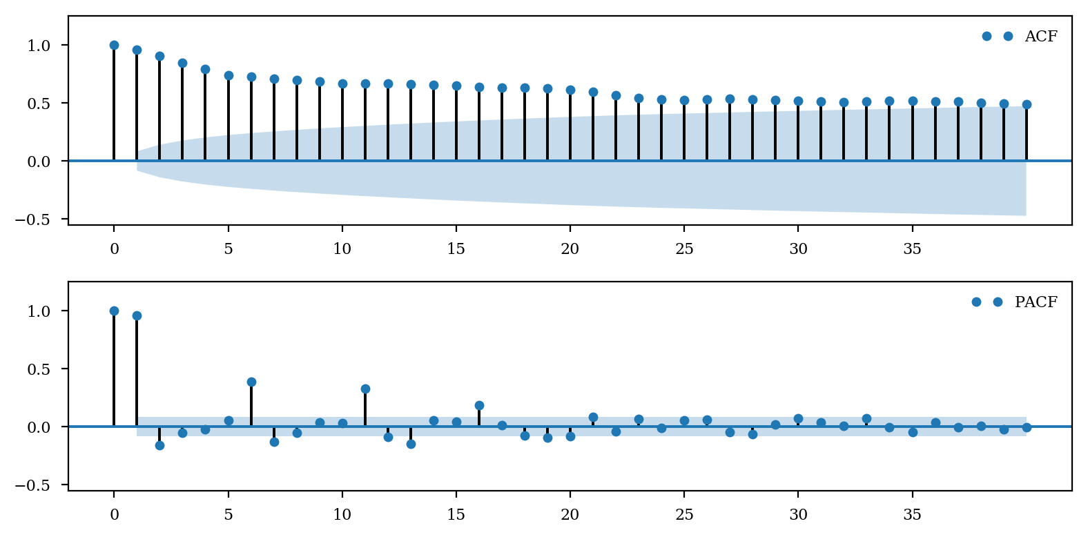
%config InlineBackend.figure_format = 'retina'
plt.close()
fig = plt.figure(figsize=(8,4))

ax1 = fig.add_subplot(211)
sm.graphics.tsa.plot_acf(train, lags=40, ax=ax1, label='ACF')
ax1.set_ylim(-.55,1.25)
ax1.set_yticks(np.arange(-.5,1.5,.5))
ax1.set_xticks(range(0,40,5))
ax1.set_title('')
handles, labels= ax1.get_legend_handles_labels()
handles = handles[:-len(handles)//3][1::2]
labels = labels[:-len(handles)//3][1::2]
ax1.legend(handles=handles, labels=labels,loc='best', frameon=0, numpoints=2)

ax2 = fig.add_subplot(212)
sm.graphics.tsa.plot_pacf(train, lags=40, ax=ax2, label='PACF')
ax2.set_ylim(-.55,1.25)
ax2.set_yticks(np.arange(-.5,1.5,.5))
ax2.set_xticks(range(0,40,5))
ax2.set_title('')
handles, labels= ax2.get_legend_handles_labels()
handles = handles[:-len(handles)//3][1::2]
labels = labels[:-len(handles)//3][1::2]
ax2.legend(handles=handles, labels=labels,loc='best', frameon=0, numpoints=2)

plt.tight_layout()
plt.savefig('uniacfpacf.pdf')
plt.show()
min_aic = min_bic = 1e5
min_aic_order = min_bic_order = (0,0)
for p in range(1,10):
    for q in range(6):
        model = sm.tsa.ARMA(train, (p, q))
        try:
            result = model.fit(trend='nc')
            stat = abs(sm.stats.durbin_watson(result.resid)-2)
            stat_score = (stat <= .01) * 3 + (.01 < stat <= .05) * 2 + (.05 < stat <= .10) * 1
            if np.abs(np.concatenate([result.arroots, result.maroots])).min() > 1.05:
                aic = result.aic
                bic = result.bic
                if aic < min_aic:
                    min_aic = aic
                    min_aic_order = (p,q)
                if bic < min_bic:
                    min_bic = bic
                    min_bic_order = (p,q)
                print('({},{}) AIC = {:>7.2f}, BIC = {:>7.2f}, |DW-2| = {:.8f} {}'.format(p,q,aic,bic,stat,stat_score*'*'))
        except:
            continue
print()
print('Minimum AIC = {:.2f} at {}, minimum BIC = {:.2f} at {}'.format(min_aic, min_aic_order, min_bic, min_bic_order))
(1,1) AIC =  113.26, BIC =  126.19, |DW-2| = 0.07497044 *
(1,2) AIC =  113.04, BIC =  130.28, |DW-2| = 0.06298702 *
(2,0) AIC =  111.43, BIC =  124.36, |DW-2| = 0.03723533 **
(2,1) AIC =  112.01, BIC =  129.25, |DW-2| = 0.04461551 **
(2,2) AIC =  113.29, BIC =  134.84, |DW-2| = 0.06107177 *
(3,0) AIC =  111.72, BIC =  128.96, |DW-2| = 0.05226283 *
(3,1) AIC =  113.64, BIC =  135.19, |DW-2| = 0.05401722 *
(4,0) AIC =  113.37, BIC =  134.92, |DW-2| = 0.05788130 *
(4,1) AIC =  115.31, BIC =  141.17, |DW-2| = 0.05672657 *
(5,0) AIC =  113.33, BIC =  139.19, |DW-2| = 0.00835075 ***

Minimum AIC = 111.43 at (2, 0), minimum BIC = 124.36 at (2, 0)
model = sm.tsa.ARMA(train, (2,0))
result = model.fit(trend='nc')
print(result.summary())
                              ARMA Model Results
==============================================================================
Dep. Variable:                  LogPs   No. Observations:                  550
Model:                     ARMA(2, 0)   Log Likelihood                 -52.713
Method:                       css-mle   S.D. of innovations              0.266
Date:                Sun, 21 May 2017   AIC                            111.426
Time:                        01:10:53   BIC                            124.355
Sample:                    07-01-2014   HQIC                           116.478
                         - 01-01-2016
===============================================================================
                  coef    std err          z      P>|z|      [0.025      0.975]
-------------------------------------------------------------------------------
ar.L1.LogPs     1.1236      0.042     26.763      0.000       1.041       1.206
ar.L2.LogPs    -0.1672      0.042     -3.976      0.000      -0.250      -0.085
                                    Roots
=============================================================================
                 Real           Imaginary           Modulus         Frequency
-----------------------------------------------------------------------------
AR.1            1.0559           +0.0000j            1.0559            0.0000
AR.2            5.6627           +0.0000j            5.6627            0.0000
-----------------------------------------------------------------------------
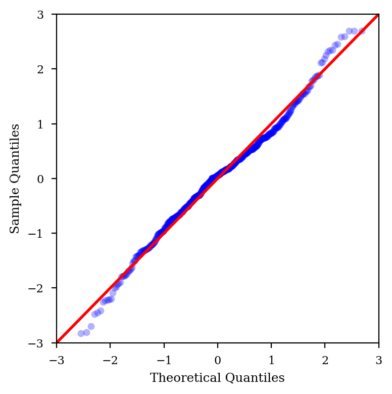
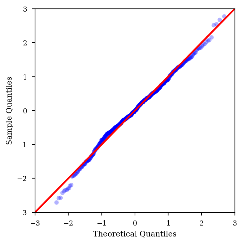
Normality test.
sm.stats.jarque_bera(result.resid)[1]
2.6180738344018359e-23
sm.stats.acorr_ljungbox(result.resid, lags=1)[1][0]
0.81633813674691746
%config InlineBackend.figure_format = 'retina'
plt.close()
fig = plt.figure(figsize=(4,4))
ax = fig.add_subplot(111)
fig = qqplot(result.resid, line='45', ax=ax, fit=True)
lines = fig.findobj(lambda x: hasattr(x, 'get_color') and x.get_color() == 'r')
dots = fig.findobj(lambda x: hasattr(x, 'get_color') and x.get_color() == 'b')
[l.set_linewidth(2) for l in lines]
[d.set_alpha(0.3) for d in dots]
# [d.set_color('c') for d in dots]
[d.set_markersize(5) for d in dots]
ax.set_ylim(-3,3)
ax.set_yticks(range(-3,4))
ax.set_xlim(-3,3)
ax.set_xticks(range(-3,4))
plt.tight_layout()
# plt.title('p-value = {}'.format(ss.normaltest(result.resid)[1]))
plt.savefig('uniqqplot.pdf')
plt.show()
phi = result.arparams * (result.pvalues[:result.k_ar]<=0.05).values

def yhat(y):  # y is now nparray of shape (k_ar,2)
    ylag = y[::-1]
    return ylag.T @ phi

fit = result.fittedvalues

pred = test * np.nan
for i in range(len(phi)):
    pred[i] = yhat(train[-1-i-len(phi):-1-i])
for i in range(len(phi), len(test)):
    pred[i] = yhat(test[i-len(phi):i])

fcst = result.forecast(len(test))
forecast = pd.Series(fcst[0], index=test.index)
conf_interval = pd.DataFrame(fcst[2], index=test.index)
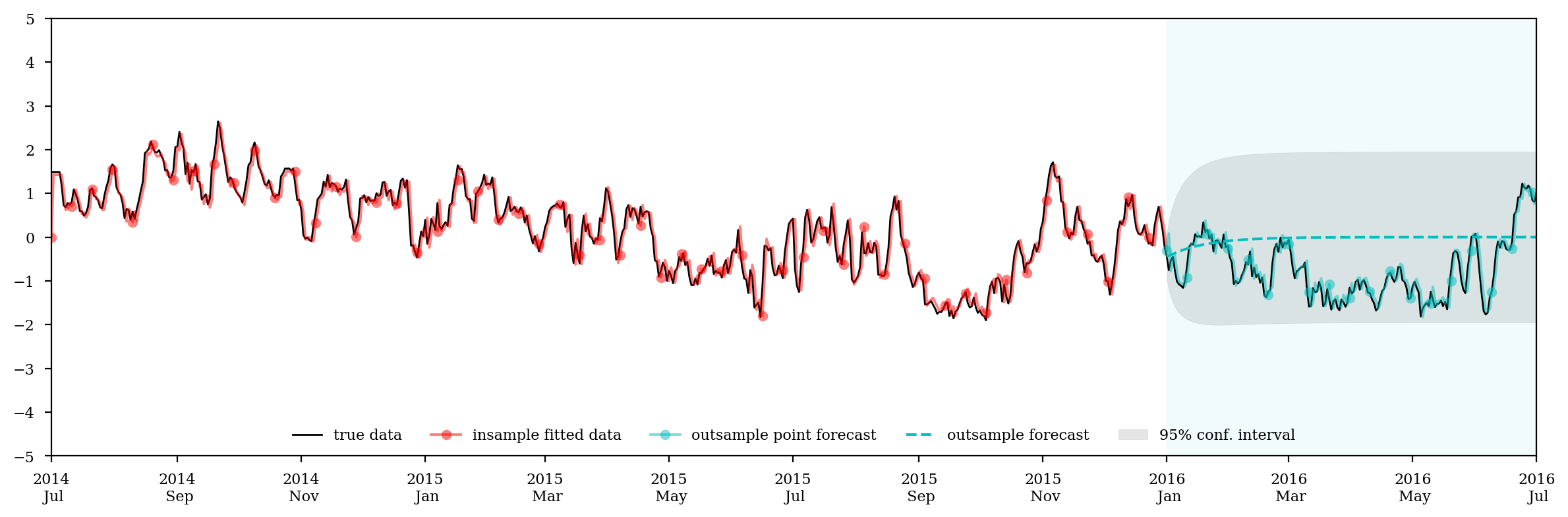
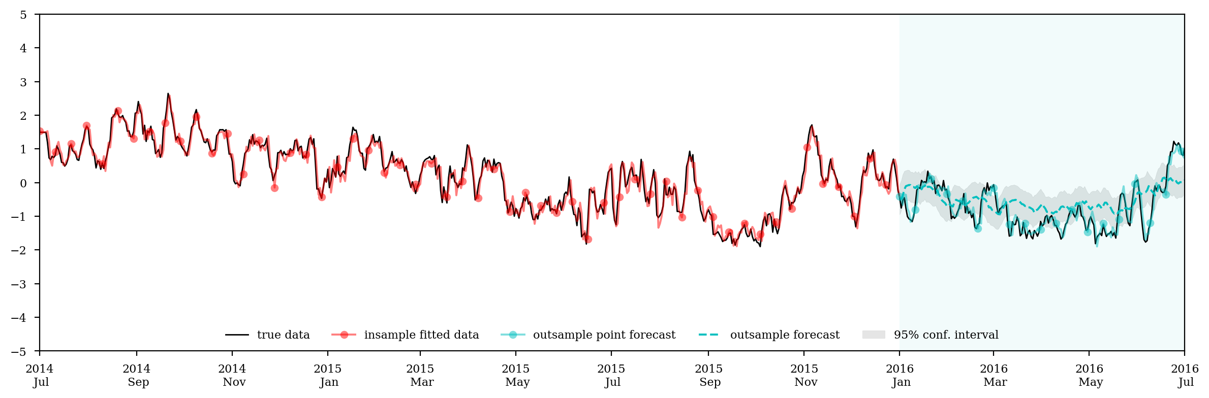
%config InlineBackend.figure_format = 'retina'
plt.close()
fig = plt.figure()
ax = fig.add_subplot(111)
ax.plot(log_price_spread, c='k',lw=1, label='true data')
ax.plot(fit, 'ro-', markevery=10, alpha=0.5, label='insample fitted data')
# ax.plot(result.fittedvalues, 'b-')
ax.plot(pred, 'co-', markevery=10, alpha=0.5, label='outsample point forecast')
ax.plot(forecast, 'c--', label='outsample forecast')
ax.axvspan(mid_date, end_date, color='c', alpha=0.05)
ax.fill_between(conf_interval.index, conf_interval.ix[:,0], conf_interval.ix[:,1], color='k', alpha=.1, label='95% conf. interval')
ax.xaxis.set_major_locator(mdates.MonthLocator(interval=2))
ax.xaxis.set_major_formatter(mdates.DateFormatter('%Y\n %b'))
ax.set_xlim(start_date, end_date)
ax.set_ylim(-5,5)
ax.set_yticks(range(-5,6))
plt.tight_layout()
plt.legend(loc='lower center', framealpha=0, ncol=5)
# plt.title('First Difference Log Price Spreads')
plt.savefig('unifit1.pdf')
plt.show()
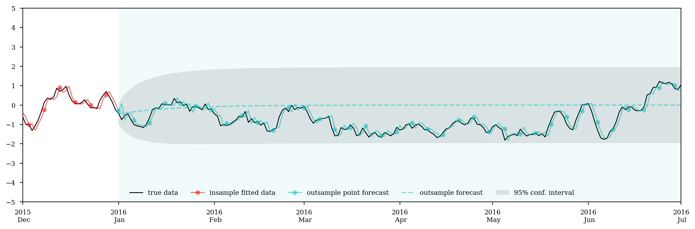
temp_date = pd.to_datetime('2015-12-01')
%config InlineBackend.figure_format = 'retina'
plt.close()
fig = plt.figure()

ax = fig.add_subplot(111)
ax.plot(log_price_spread, c='k',lw=1, label='true data')
ax.plot(fit, 'ro-', markevery=5, alpha=0.5, label='insample fitted data')
ax.plot(pred, 'co-', markevery=5, alpha=0.5, label='outsample point forecast')
ax.plot(forecast, 'c--', alpha=0.5, label='outsample forecast')
ax.axvspan(mid_date, end_date, color='c', alpha=0.05)
ax.fill_between(conf_interval.index, conf_interval.ix[:,0], conf_interval.ix[:,1], color='k', alpha=.1, label='95% conf. interval')
ax.xaxis.set_major_locator(mdates.MonthLocator(interval=1))
ax.xaxis.set_major_formatter(mdates.DateFormatter('%Y\n %b'))
ax.set_xlim(temp_date, end_date)
ax.set_ylim(-5,5)
ax.set_yticks(range(-5,6))
plt.tight_layout()
plt.legend(loc='lower center', framealpha=0, ncol=5)
# plt.title('First Difference Log Price Spreads')
plt.savefig('unifit2.pdf')
plt.show()
MASE (Mean Absolute Scaled Error): https://en.wikipedia.org/wiki/Mean_absolute_scaled_error
- Better than MAPE: MASE is symmetric while MAPE punishes on negative errors
- Better than RMSE: scaled to the data
- Better than R-squares: parameter number irrelavant
- Better than AUC and Predictive Likelihood: easier to compute
def mase(data, pred):
    error = data - pred
    ydiff = data.diff().dropna()
    return error.abs().mean() / ydiff.abs().mean()
mase_uni_is = mase(train, fit)
mase_uni_osp = mase(test, pred)
mase_uni_os = mase(test, forecast)
print('MASE insample is {:.3f}'.format(mase_uni_is))
print('MASE outsample point is {:.3f}'.format(mase_uni_osp))
print('MASE outsample is {:.3f}'.format(mase_uni_os))
MASE insample is 0.996
MASE outsample point is 0.991
MASE outsample is 4.704
Step 5: Multivariate Model - ARIMAX(p,d,q)
data = [
    'BCHAIN/ATRCT',     # Bitcoin Median Transaction Confirmation Time
    'BCHAIN/CPTRA',     # Bitcoin Cost Per Transaction
    'BCHAIN/DIFF',      # Bitcoin Mining Difficulty
    'BCHAIN/TVTVR',     # Bitcoin Trade Volume vs Transaction Volume Ratio
]
ind = [quandl.get(d)[start_date:end_date] for d in data]
max_volume = ((volume.apply(lambda v:v.index, axis=1).T == max_exchange.apply(lambda i:exchangelist[i])).T * volume).sum(axis=1)
min_volume = ((volume.apply(lambda v:v.index, axis=1).T == min_exchange.apply(lambda i:exchangelist[i])).T * volume).sum(axis=1)
trade_volume = max_volume + min_volume
transaction_volume = (trade_volume * ind[-1].T).T
ind[-1] = transfer_volume = transaction_volume.Value - trade_volume
dataset = pd.concat([price_spread, trade_volume] + ind, axis=1, join='outer')
dataset.columns = ['Ps', 'Tr', 'Ct', 'Co', 'Di', 'Tf']
print(dataset.describe())
               Ps           Tr          Ct          Co            Di             Tf
count  732.000000   732.000000  732.000000  732.000000  7.320000e+02     732.000000
mean     7.418801   727.610416    8.056266   12.379825  7.563867e+10   22286.774041
std      7.705870   243.943093    1.111682    8.532508  5.491585e+10   23071.094095
min      0.150000   356.410000    5.883333    3.442916  1.681846e+10    1057.026608
25%      2.430000   499.281875    7.333333    7.574733  4.055572e+10    7382.009772
50%      4.914920   713.810010    7.875000    8.890402  4.969239e+10   12993.766448
75%      9.461703   864.820000    8.600000   13.035012  9.605659e+10   29144.912952
max     78.191470  1532.508000   14.130000   49.667654  2.094532e+11  136972.126998
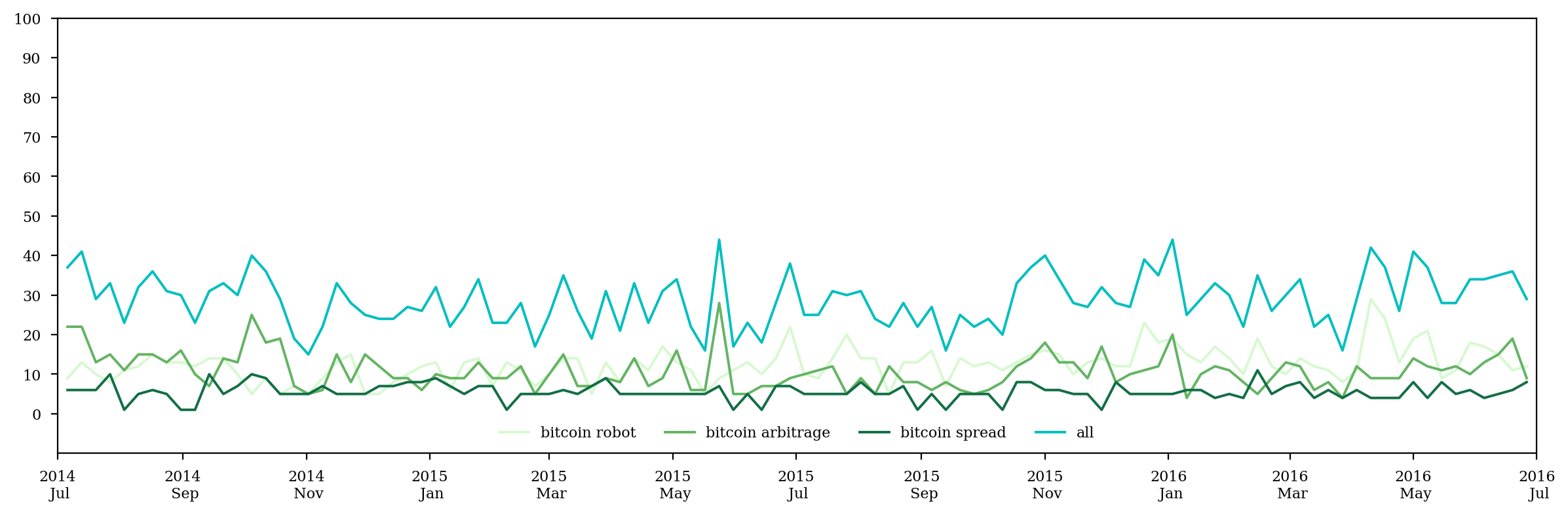
googletrends = []
kw_list = ['bitcoin robot', 'bitcoin arbitrage', 'bitcoin spread']
pytrend.build_payload(kw_list=kw_list)
googletrends = pytrend.interest_over_time().ix[start_date:end_date, :] + 1  # as googletrends can be 0 from time to time, which is troublesome for taking log
plt.close()
fig = plt.figure()
ax = fig.add_subplot(111)
for i in range(len(kw_list)):
    ax.plot(googletrends.ix[:,i], c=cmocean.cm.algae(i/len(kw_list)), label=kw_list[i])
ax.plot(googletrends.sum(axis=1), c='c', label='all')
ax.xaxis.set_major_locator(mdates.MonthLocator(interval=2))
ax.xaxis.set_major_formatter(mdates.DateFormatter('%Y\n %b'))
ax.set_xlim(start_date, end_date)
plt.tight_layout()
plt.legend(loc='lower center', frameon=0, ncol=len(kw_list)+1)
plt.ylim(-10,100)
plt.yticks(range(0,101,10))
plt.savefig('multrend.pdf')
plt.show()
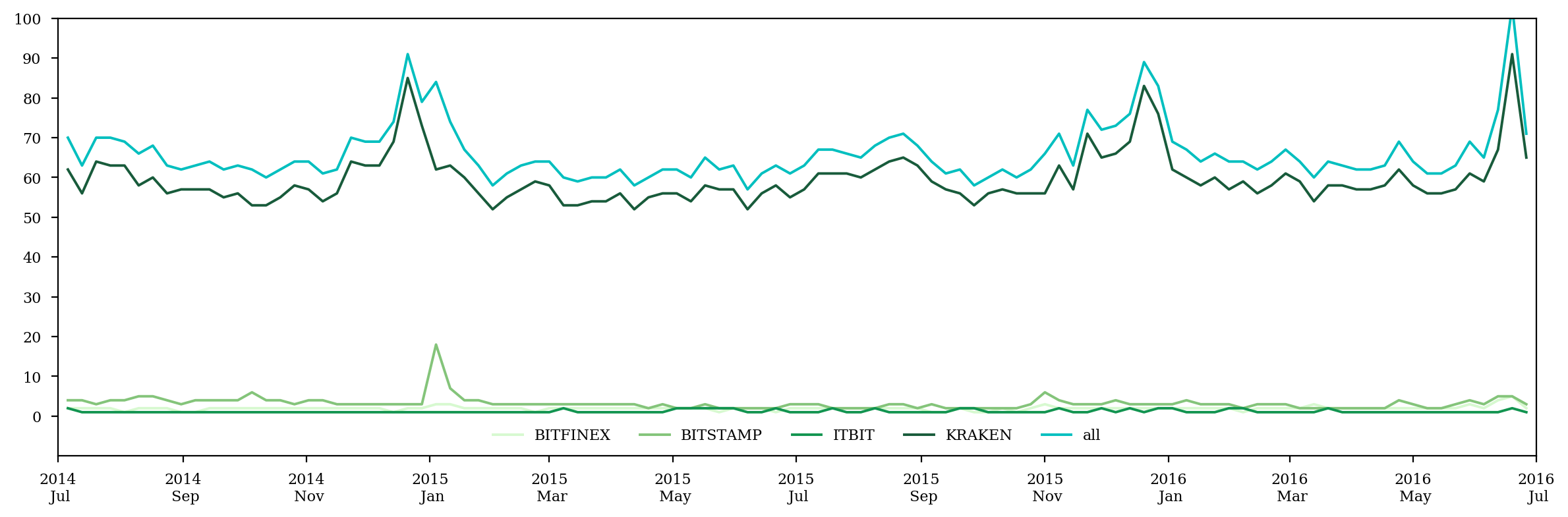
exchangetrends = []
kw_list = np.setdiff1d(exchangelist, ['ROCK'])
pytrend.build_payload(kw_list=kw_list)
exchangetrends = pytrend.interest_over_time().ix[start_date:end_date, :] + 1
plt.close()
fig = plt.figure()
ax = fig.add_subplot(111)
for i in range(len(kw_list)):
    ax.plot(exchangetrends.ix[:,i], color=cmocean.cm.algae(i/len(kw_list)), label=kw_list[i])
ax.plot(exchangetrends.sum(axis=1), c='c', label='all')
ax.xaxis.set_major_locator(mdates.MonthLocator(interval=2))
ax.xaxis.set_major_formatter(mdates.DateFormatter('%Y\n %b'))
ax.set_xlim(start_date, end_date)
plt.tight_layout()
plt.legend(loc='lower center', frameon=0, ncol=len(kw_list)+1)
plt.ylim(-10,100)
plt.yticks(range(0,101,10))
plt.savefig('multrend.pdf')
plt.show()
dataset = pd.concat([dataset, googletrends.sum(axis=1), exchangetrends.sum(axis=1)], axis=1, join='outer').fillna(method='ffill').fillna(method='bfill')
dataset.columns = list(dataset.columns[:-2]) + ['Gt1', 'Gt2']
dataset.Gt1.interpolate(inplace=1)
dataset.Gt2.interpolate(inplace=1)
log_dataset = z_norm(np.log(dataset).rolling(5).mean().fillna(method='bfill'))
log_dataset.columns = ['Log'+c for c in log_dataset.columns]
print(log_dataset.describe())
              LogPs         LogTr         LogCt         LogCo         LogDi         LogTf        LogGt1        LogGt2
count  7.320000e+02  7.320000e+02  7.320000e+02  7.320000e+02  7.320000e+02  7.320000e+02  7.320000e+02  7.320000e+02
mean  -4.284976e-15  1.526951e-14  2.660744e-14 -2.311827e-16  5.078330e-14 -1.000566e-14  4.753939e-15  9.735989e-15
std    1.000000e+00  1.000000e+00  1.000000e+00  1.000000e+00  1.000000e+00  1.000000e+00  1.000000e+00  1.000000e+00
min   -1.902323e+00 -1.600349e+00 -2.681378e+00 -1.602305e+00 -1.918163e+00 -2.449733e+00 -2.868102e+00 -1.541291e+00
25%   -8.414662e-01 -1.003732e+00 -6.189083e-01 -6.491453e-01 -5.965383e-01 -7.432149e-01 -6.731405e-01 -6.369187e-01
50%   -1.734537e-02  8.771289e-02 -2.819185e-02 -4.128926e-01 -2.796970e-01 -1.754303e-01  4.339693e-02 -2.954394e-01
75%    7.996859e-01  6.973955e-01  5.295034e-01  4.580167e-01  6.834602e-01  6.506610e-01  7.555832e-01  4.566839e-01
max    2.645812e+00  2.439251e+00  3.834172e+00  2.765270e+00  1.896075e+00  2.321454e+00  2.077746e+00  4.822614e+00
%config InlineBackend.figure_format = 'retina'
plt.close()

fig = plt.figure(figsize=(5,4))

ax = fig.add_subplot(111)
idx = log_dataset.corr().sort_values(by='LogPs', ascending=0).index
log_dataset = log_dataset.ix[:,idx]
corr = log_dataset.corr()
sns.heatmap(corr, square=1, ax=ax)

plt.yticks(rotation=0)
plt.xticks(rotation=90)

plt.tight_layout()
plt.savefig('mulcorr.pdf')
plt.show()
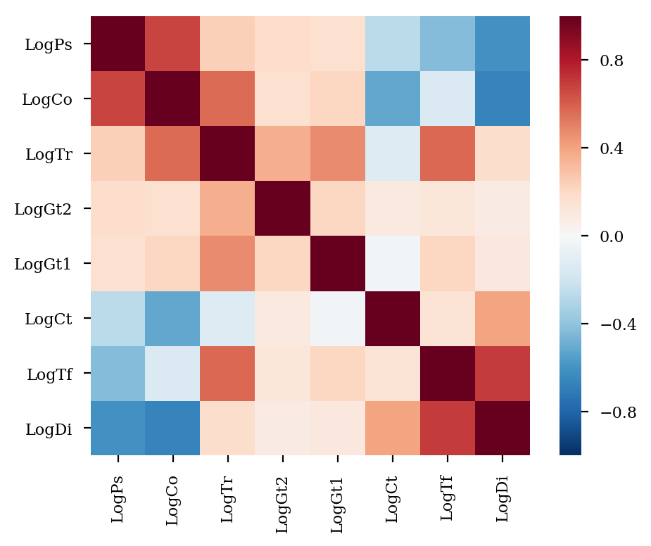
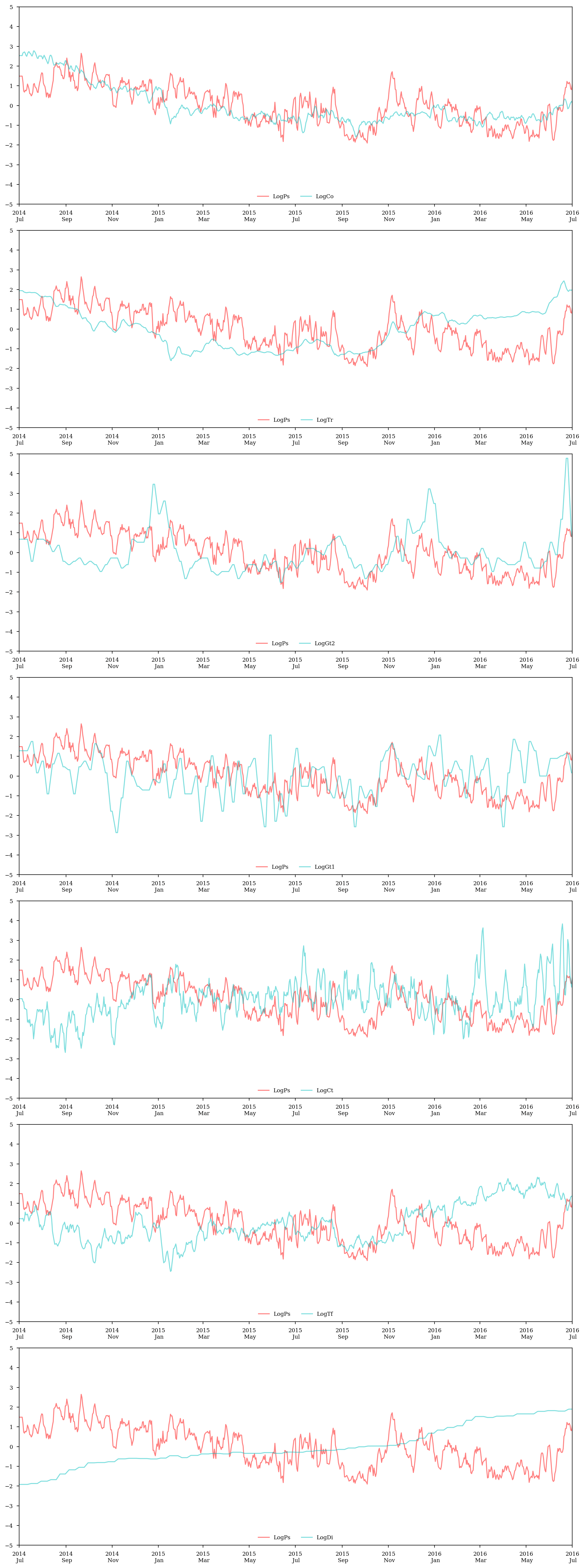
fig = plt.figure(figsize=(12,4*len(corr)))
for i in range(len(corr)-1):
    ax = fig.add_subplot(len(corr)-1,1,i+1)
    ax.plot(log_price_spread, c='r', label='LogPs', alpha=.5)
    ax.plot(log_dataset.ix[:,i+1], c='c', alpha=.5, label=log_dataset.columns[i+1])
    ax.legend(frameon=0,loc='lower center', ncol=2)
    ax.xaxis.set_major_locator(mdates.MonthLocator(interval=2))
    ax.xaxis.set_major_formatter(mdates.DateFormatter('%Y\n %b'))
    ax.set_xlim(start_date, end_date)
    ax.set_ylim(-5,5)
    ax.set_yticks(range(-5,6))
plt.tight_layout()
plt.show()
endog = log_dataset.LogPs
exog = log_dataset.ix[:,np.setdiff1d(log_dataset.columns,['LogPs'])]
train_endog = endog.ix[start_date:mid_date]
train_exog = exog.ix[start_date:mid_date]
test_endog = endog.ix[mid_date:end_date]
test_exog = exog.ix[mid_date:end_date]
min_aic = min_bic = 1e5
min_aic_order = min_bic_order = (0,0,0)
for p in range(1,10):
    for q in range(3):
        for d in range(1):
            model = sm.tsa.SARIMAX(train_endog, train_exog, (p, d, q))
            try:
                result = model.fit(trend='nc')
                result.summary()
            except:
                continue
            stat = abs(sm.stats.durbin_watson(result.resid)-2)
            stat_score = (stat <= 0.01) * 3 + (0.01 < stat <= 0.05) * 2 + (0.05 < stat <= 0.10) * 1
            if np.abs(np.concatenate([result.arroots, result.maroots])).min() > 1.05:
                aic = result.aic
                bic = result.bic
                if aic < min_aic:
                    min_aic = aic
                    min_aic_order = (p,d,q)
                if bic < min_bic:
                    min_bic = bic
                    min_bic_order = (p,d,q)
                print('({},{},{}) AIC = {:>7.2f}, BIC = {:>7.2f}, |DW-2| = {:.8f} {}'.format(p,d,q,aic,bic,stat,stat_score*'*'))
print()
print('Minimum AIC = {:.2f} at {}, minimum BIC = {:.2f} at {}'.format(min_aic, min_aic_order, min_bic, min_bic_order))
(1,0,0) AIC =   95.23, BIC =  134.02, |DW-2| = 0.32750528
(1,0,1) AIC =   82.47, BIC =  125.56, |DW-2| = 0.03040248 **
(1,0,2) AIC =   81.51, BIC =  128.92, |DW-2| = 0.01859667 **
(2,0,0) AIC =   79.67, BIC =  122.77, |DW-2| = 0.02601878 **
(2,0,1) AIC =   77.37, BIC =  124.78, |DW-2| = 0.02101876 **
(2,0,2) AIC =   77.46, BIC =  129.18, |DW-2| = 0.02477762 **
(3,0,0) AIC =   77.69, BIC =  125.10, |DW-2| = 0.00997169 ***
(3,0,1) AIC =   75.14, BIC =  126.85, |DW-2| = 0.00109986 ***
(4,0,0) AIC =   75.70, BIC =  127.42, |DW-2| = 0.00565012 ***
(4,0,1) AIC =   77.69, BIC =  133.72, |DW-2| = 0.00489150 ***
(5,0,0) AIC =   77.64, BIC =  133.67, |DW-2| = 0.00382267 ***
(5,0,1) AIC =   56.67, BIC =  117.01, |DW-2| = 0.11066651
(6,0,0) AIC =  -11.64, BIC =   48.69, |DW-2| = 0.10243475
(6,0,1) AIC =  -16.11, BIC =   48.54, |DW-2| = 0.02155382 **
(6,0,2) AIC =  -16.40, BIC =   52.56, |DW-2| = 0.00558554 ***
(7,0,0) AIC =  -18.40, BIC =   46.25, |DW-2| = 0.00766101 ***
(7,0,1) AIC =  -16.75, BIC =   52.20, |DW-2| = 0.00203650 ***
(7,0,2) AIC =  -15.06, BIC =   58.20, |DW-2| = 0.00505927 ***
(8,0,0) AIC =  -17.85, BIC =   51.11, |DW-2| = 0.00599037 ***
(8,0,1) AIC =  -21.57, BIC =   51.70, |DW-2| = 0.01490724 **
(8,0,2) AIC =  -18.89, BIC =   58.69, |DW-2| = 0.02765866 **
(9,0,0) AIC =  -15.87, BIC =   57.40, |DW-2| = 0.00530673 ***
(9,0,1) AIC =  -20.02, BIC =   57.56, |DW-2| = 0.00183866 ***
(9,0,2) AIC =  -17.87, BIC =   64.01, |DW-2| = 0.01105891 **

Minimum AIC = -21.57 at (8, 0, 1), minimum BIC = 46.25 at (7, 0, 0)
model = sm.tsa.SARIMAX(train_endog, train_exog, (8,0,1), freq='D')
result = model.fit(trend='nc')
print(result.summary())
                           Statespace Model Results
==============================================================================
Dep. Variable:                  LogPs   No. Observations:                  550
Model:               SARIMAX(8, 0, 1)   Log Likelihood                  27.783
Date:                Sun, 21 May 2017   AIC                            -21.566
Time:                        01:13:14   BIC                             51.703
Sample:                    07-01-2014   HQIC                             7.066
                         - 01-01-2016
Covariance Type:                  opg
==============================================================================
                 coef    std err          z      P>|z|      [0.025      0.975]
------------------------------------------------------------------------------
LogCo          0.3659      0.181      2.024      0.043       0.012       0.720
LogCt          0.0089      0.039      0.224      0.823      -0.069       0.086
LogDi         -0.0414      0.266     -0.156      0.876      -0.563       0.480
LogGt1         0.0069      0.061      0.113      0.910      -0.113       0.127
LogGt2        -0.0132      0.084     -0.157      0.875      -0.178       0.152
LogTf         -0.3987      0.087     -4.557      0.000      -0.570      -0.227
LogTr          0.3262      0.180      1.815      0.069      -0.026       0.678
ar.L1          0.3475      0.168      2.063      0.039       0.017       0.678
ar.L2          0.7677      0.183      4.200      0.000       0.409       1.126
ar.L3         -0.1169      0.054     -2.171      0.030      -0.222      -0.011
ar.L4         -0.0721      0.051     -1.402      0.161      -0.173       0.029
ar.L5         -0.4598      0.047     -9.752      0.000      -0.552      -0.367
ar.L6          0.2162      0.088      2.468      0.014       0.045       0.388
ar.L7          0.3528      0.077      4.600      0.000       0.202       0.503
ar.L8         -0.1733      0.044     -3.953      0.000      -0.259      -0.087
ma.L1          0.7612      0.174      4.369      0.000       0.420       1.103
sigma2         0.0526      0.003     18.715      0.000       0.047       0.058
===================================================================================
Ljung-Box (Q):                      138.21   Jarque-Bera (JB):                28.29
Prob(Q):                              0.00   Prob(JB):                         0.00
Heteroskedasticity (H):               1.54   Skew:                            -0.30
Prob(H) (two-sided):                  0.00   Kurtosis:                         3.93
===================================================================================

Warnings:
[1] Covariance matrix calculated using the outer product of gradients (complex-step).
sm.stats.durbin_watson(result.resid)
1.9750927630586519
sm.stats.jarque_bera(result.resid)[1]
7.8859408081166919e-07
sm.stats.acorr_ljungbox(result.resid, lags=1)[1][0]
0.87455062641970893
%config InlineBackend.figure_format = 'retina'
plt.close()
fig = plt.figure(figsize=(4,4))
ax = fig.add_subplot(111)
fig = qqplot(result.resid, line='45', ax=ax, fit=True)
lines = fig.findobj(lambda x: hasattr(x, 'get_color') and x.get_color() == 'r')
dots = fig.findobj(lambda x: hasattr(x, 'get_color') and x.get_color() == 'b')
[l.set_linewidth(2) for l in lines]
[d.set_alpha(0.3) for d in dots]
[d.set_markersize(5) for d in dots]
ax.set_ylim(-3,3)
ax.set_yticks(range(-3,4))
ax.set_xlim(-3,3)
ax.set_xticks(range(-3,4))
plt.tight_layout()
# plt.title('p-value = {}'.format(ss.normaltest(result.resid)[1]))
plt.savefig('mulqqplot.pdf')
plt.show()
forecast = result.forecast(steps=len(test_endog), exog=test_exog)
fit = result.fittedvalues

model = sm.tsa.statespace.SARIMAX(endog, exog, model.order)
result = model.filter(result.params)
predict = result.get_prediction()
pred = predict.predicted_mean[mid_date:]
conf_interval = [forecast+predict.se_mean[len(train_endog):]*1.96,forecast-predict.se_mean[len(train_endog):]*1.96]
%config InlineBackend.figure_format = 'retina'
plt.close()
fig = plt.figure()
ax = fig.add_subplot(111)
ax.plot(log_price_spread, c='k',lw=1, label='true data')
ax.plot(fit, 'ro-', markevery=10, alpha=0.5, label='insample fitted data')
ax.plot(pred, 'co-', markevery=10, alpha=0.5, label='outsample point forecast')
ax.plot(forecast, 'c--', label='outsample forecast')
ax.axvspan(mid_date, end_date, color='c', alpha=0.05)
ax.fill_between(test_endog.index, conf_interval[0], conf_interval[1], color='k', alpha=.1, label='95% conf. interval')
ax.xaxis.set_major_locator(mdates.MonthLocator(interval=2))
ax.xaxis.set_major_formatter(mdates.DateFormatter('%Y\n %b'))
ax.set_xlim(start_date, end_date)
ax.set_ylim(-5,5)
ax.set_yticks(range(-5,6))
plt.tight_layout()
plt.legend(loc='lower center', framealpha=0, ncol=5)
# plt.title('First Difference Log Price Spreads')
plt.savefig('mulfit1.pdf')
plt.show()
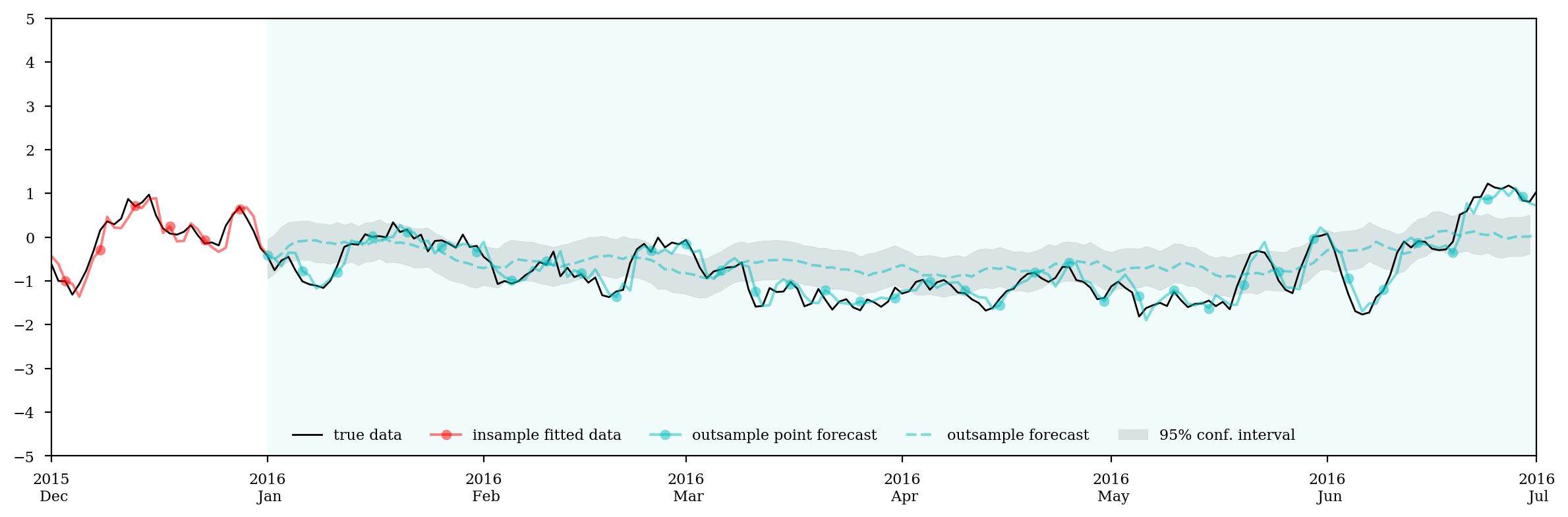
%config InlineBackend.figure_format = 'retina'
plt.close()
fig = plt.figure()

ax = fig.add_subplot(111)
ax.plot(log_price_spread, c='k',lw=1, label='true data')
ax.plot(fit, 'ro-', markevery=5, alpha=0.5, label='insample fitted data')
ax.plot(pred, 'co-', markevery=5, alpha=0.5, label='outsample point forecast')
ax.plot(forecast, 'c--', alpha=0.5, label='outsample forecast')
ax.axvspan(mid_date, end_date, color='c', alpha=0.05)
ax.fill_between(test_endog.index, conf_interval[0], conf_interval[1], color='k', alpha=.1, label='95% conf. interval')
ax.xaxis.set_major_locator(mdates.MonthLocator(interval=1))
ax.xaxis.set_major_formatter(mdates.DateFormatter('%Y\n %b'))
ax.set_xlim(temp_date, end_date)
ax.set_ylim(-5,5)
ax.set_yticks(range(-5,6))
plt.tight_layout()
plt.legend(loc='lower center', framealpha=0, ncol=5)
# plt.title('First Difference Log Price Spreads')
plt.savefig('mulfit2.pdf')

plt.show()
mase_mul_is = mase(train_endog, fit)
mase_mul_osp = mase(test_endog, pred)
mase_mul_os = mase(test_endog, forecast)
print('MASE insample is {:.3f}'.format(mase_mul_is))
print('MASE outsample is {:.3f}'.format(mase_mul_osp))
print('MASE outsample is {:.3f}'.format(mase_mul_os))
MASE insample is 0.858
MASE outsample is 0.857
MASE outsample is 2.688
uni = np.array([mase_uni_is, mase_uni_osp, mase_uni_os])
mul = np.array([mase_mul_is, mase_mul_osp, mase_mul_os])
print(uni)
print(mul)
[ 0.99605648  0.99134227  4.70378576]
[ 0.8576784   0.85705027  2.68798458]
plt.figure(figsize=(8,4))
plt.plot((0,0),(0,5),'#eeeeee',ls='--')
plt.plot((1,1),(0,5),'#eeeeee',ls='--')
plt.plot((2,2),(0,5),'#eeeeee',ls='--')
plt.plot(uni, 'ro-', label='univariate model')
plt.plot(mul, 'ko-', label='multivariate model')
plt.legend(loc='lower center', frameon=0, ncol=2)
plt.xticks(range(3),['insample', 'outsample point', 'outsample'])
# plt.title('MASE Scores')
plt.yticks(np.arange(0,6))
plt.ylim(0,5)
plt.tight_layout()
plt.savefig('mase.pdf')
plt.show()
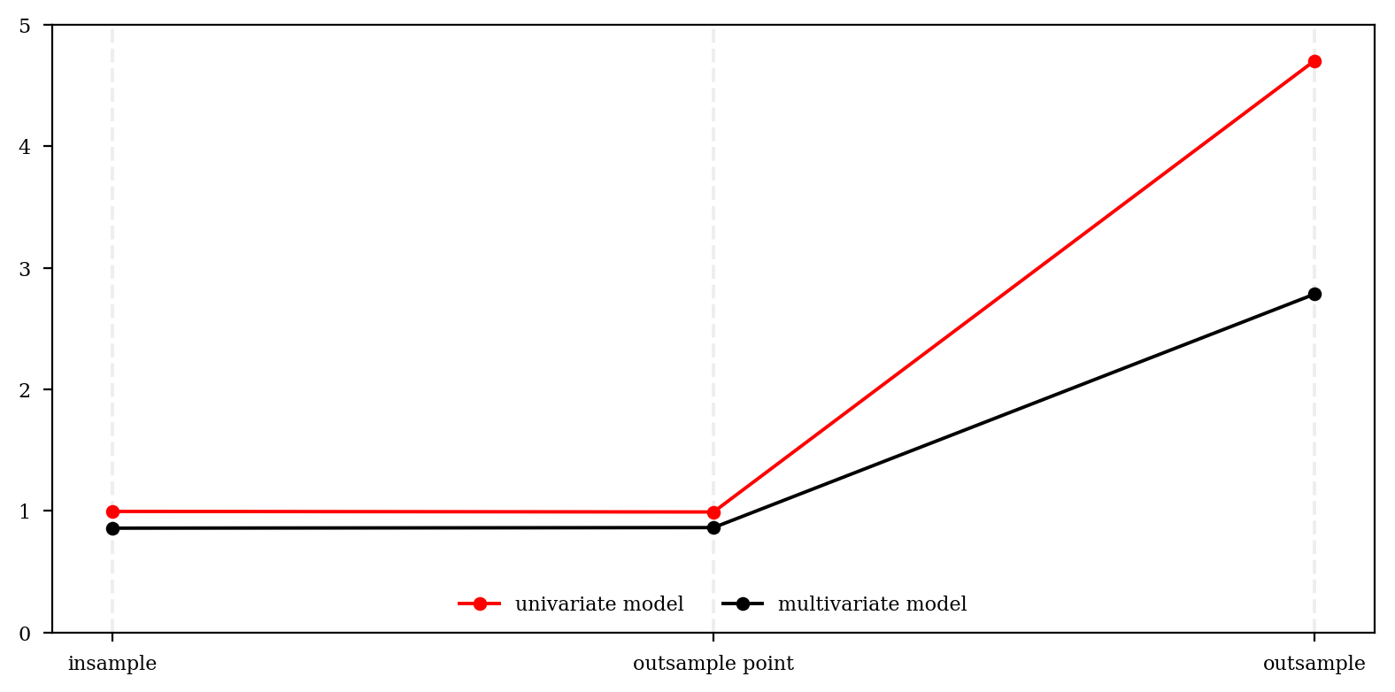
Step 6: Conclusion
So our exogenous indicators do work. We’ll see what else we can do with the multivariate model next time.