Notes on Operations Research
2017-03-27
This is my lecture notes from the course Operations Research. The course was intended to be a fundamental one introducing various aspects of operations research, the thinking process of a typical optimization problem, and famous theorems and applications.
Introduction
- Summary of this lecture:
- Introduction
- Basic Linear Programming
- Taha Chapters 1, 2, 3
- Structure:
- 7 lectures
- 7 tutorials
- 2 assignments
- individual written open-book exam (only book and no notes in the book)
- Operations Research definition:
- In short: OR is the discipline of applying advanced analytical methods to help make better decisions.
- Performing an OR project:
- Problem definition
- Data collection
- Type of input data
- Options to use data
- Making assumptions
- Modeling Terminology: parameters, decision variables, objective, constraints
- Model design and implementation
- Algorithms
- Definition: step-by-step procedure for solving a problem to optimality
- Techniques:
- Enumeration
- Improvement approach
- Search algorithms
- Dynamic Programming
- Performance of an algorithm
- Metric: TIME TO FIND OPTIMAL SOLUTION
- Practical: NUMBER OF STEPS
- Approaches:
- Empirical analysis
- Average-case analysis
- Worst-case analysis
- Time complexity
- Example: Traveling Salesman Problem (TSP)
- An optimal algorithm is by enumeration:
$(n-1)!/2$solutions
- An optimal algorithm is by enumeration:
- Heuristics 启发式算法
- Definition:
- A heuristic aims at finding good, but not necessarily optimal, feasible solutions
- Metrics:
- Generates objective values close to optimality
- Simplicity
- Speed
- Robustness
- Good stopping criteria
- Produce multiple solutions
- Testing quality of heurisics
- TSP example: nearest neighbor heuristic
- Definition:
Basic Linear Programming (LP)
- Notation
- Maximum
- Hyperplanes, Halfspaces & Polyhedrons
- Corner point feasible solutions
- Simplex method
- Check LP properties:
- Proportionality
- Additivity
- Divisibility
- Certainty
- Fixing format
- Always “max”
- All right-hand side must be non-negative
- All functional constraints are equalities
- All variables on the left, and constants on the right
- All decisive variables are non-negative
- FINALLY: we get
$\text{max}\sum x_i\qquad\text{s.t.}\sum x_{i_k}=b_k,\quad x_i\ge 0$ - HOWEVER: we need to assure all-zero is feasible for original variables and thus we introduce artificial variables. This draws out the “big-M” method
- Entering & leaving basic variable
- Properties
- If there is exactly one optimal solution, then it must be a CPF solution. 反证法
- If there are multiple optimal solutions then at least two must be adjacent CPF solutions (provided we have a bounded feasible region).
- The number of CPF solutions is bounded from above by
$\begin{pmatrix}m+n\\ n\end{pmatrix}$ - If a CPF has no adjacent CPF solutions that are better, then there are no better CPF solutions anywhere.
- Basic & basic feasible solutions: among all
$m+n$variables- A basic solution is where
$n$constraints hold with equality ($\mathbf{a}_i^T\mathbf{x}=\mathbf{b}_i$or$x_j=0$). So there are$m$basic variables and$n$nonbasic variables (that are all set zero). - A basic feasible solution is where
$n$constraints hold with equality and all other constraints are satisfied. So there are$m$basic variables that are nonnegative.
- A basic solution is where
- Equation form
- Original constraint:
$\mathbf{a}_i^T\mathbf{x}\le b_i$ - Equation form:
$\mathbf{a}_i^T\mathbf{x}+x_{n+i}=b_i$ $x_{n+i}$is called indicating variable
- Original constraint:
- Check LP properties:
- Comparison
| Particulars | Slack Variable | Surplus Variable | Artificial Variable |
|---|---|---|---|
| Mean | Unused idle resources. | Excess utilized resources. | No physical or economic meaning. |
| When used | With < Constraints | With > constraints | With ≥ constraints |
| Coefficient | +1 | −1 | +1 |
| Coef. in obj. | 0 | 0 | −M for max, +M for min |
| As initial program variable | Used as starting point. | Can’t be used since unit matrix condition is not satisfied | It is initially used but later on eliminated. |
| In optimal table | Used to help for interpreting idle & key resources. | – | It indicates the infeasible solution |
Matrix Notation
- Notation
-
Constraints: From
$\text{max }Z=\sum_{i=1}^nc_ix_i\text{ s.t. }\sum_{i=1}^na_{ji}x_i\le b_i$to$$ \begin{aligned} & \text{max }Z=c^Tx\\ & \text{s.t. } \begin{bmatrix} \mathbf{A} & \mathbf{I} \end{bmatrix} \begin{bmatrix}x\\ x_s\end{bmatrix}=b,\begin{bmatrix}x\\ x_s\end{bmatrix}\ge0 \end{aligned} $$ -
Simplex tableau as matrix: generally
$$ \begin{bmatrix} \mathbf{A} & \mathbf{I} \end{bmatrix} \begin{bmatrix} x\\ x_s \end{bmatrix}=b \qquad \text{or}\qquad \begin{bmatrix} 1 & -c^T & 0\\ 0 & \mathbf{A} & \mathbf{I} \end{bmatrix} \begin{bmatrix} Z\\ x\\ x_s \end{bmatrix} = \begin{bmatrix} 0\\ b \end{bmatrix} $$while we can simplify
$$ \begin{bmatrix} \mathbf{A} & \mathbf{I} \end{bmatrix} \begin{bmatrix} x\ x_s \end{bmatrix}=b $$
to
$$ \mathbf{Bx_B}=b $$
which we solve by
$$ \mathbf{x_B}=\mathbf{B}^{-1}b $$
and
$$ Z=c_B^T\mathbf{x_B}=c_B^T\mathbf{B}^{-1}b $$
so further more, we may find that
$$ \begin{bmatrix} 1 & -c^T & 0\\ 0 & \mathbf{A} & \mathbf{I} \end{bmatrix} \begin{bmatrix} Z\\ x\\ x_s \end{bmatrix} = \begin{bmatrix} 0\\ b \end{bmatrix} $$can be rewritten by iteration into
$$ \begin{bmatrix} 1 & c_B^TB^{-1}A-c^T & c_B^TB^{-1}\\ 0 & B^{-1}A & B^{-1} \end{bmatrix} \begin{bmatrix} Z\\ x\\ x_s \end{bmatrix} = \begin{bmatrix} c_B^TB^{-1}b\\ B^{-1}b \end{bmatrix} $$ -
Basic variables are those set non-zero. They are at first slack and artificial variables.
-
Example of Simplex method
Consider the following problem:$$ \begin{aligned} &\text{min }Z=3x_1+2x_2\\ &\text{s.t. } \begin{cases} 2x_1+x_2\ge 10\\ -3x_1+2x_2\le 6\\ x_1+x_2\ge 6\ x_1\ge 0,x_2\ge 0 \end{cases} \end{aligned} $$
Now use the Simplex method in matrix notation to solve it. First, convert the problem to equation form
$$ \begin{aligned} &\text{max }Z=-3x_1-2x_2\\ &\text{s.t. } \begin{cases} 2x_1 &+ x_2 &- x_3 & & &= 10\\ -3x_1 &+ 2x_2 & & &+ x_5 &= 6 \\ x_1 &+ x_2 & &- x_4 & &=6\\ x_1\ge 0 & x_2\ge 0 & x_3\ge 0 & x_4\ge 0 & x_5\ge 0 \end{cases} \end{aligned} $$where
$x_3$,$x_4$are here surplus variables, while$x_5$is a slack variable. So later on we may use$x_5$as an initial variable. Use big-M to ensure that if all original variables are set zero, we still have a feasible starting solution$$ \begin{aligned} &\text{max }Z=-3x_1-2x_2-Mx_6-Mx_7\\ &\text{s.t. } \begin{cases} 2x_1 &+ x_2 &- x_3 & & &+ x_6 & &= 10\\ -3x_1 &+ 2x_2 & & &+ x_5 & & &= 6 \\ x_1 &+ x_2 & &- x_4 & & &+ x_7 &=6\\ x_1\ge 0 & x_2\ge 0 & x_3\ge 0 & x_4\ge 0 & x_5\ge 0 & & \end{cases} \end{aligned} $$where
$x_6$and$x_7$are artificial variables, and thus will be used as initial variables. Now write in matrix form$$ \begin{bmatrix} 1 & 3 & 2 & 0 & 0 & 0 & M & M\\ 0 & 2 & 1 & -1 & 0 & 0 & 1 & 0\\ 0 & -3 & 2 & 0 & 0 & 1 & 0 & 0\\ 0 & 1 & 1 & 0 & - & 0 & 0 & 1 \end{bmatrix} \begin{bmatrix} Z\\ x_1\\ x_2\\ x_3\\ x_4\\ x_5\\ x_6\\ x_7 \end{bmatrix}= \begin{bmatrix} 0\\ 10\\ 6\\ 6 \end{bmatrix} $$In shorthand notation (Simplex tableau)
$$ \begin{bmatrix} 1 & 3 & 2 & 0 & 0 & 0 & M & M\\ 0 & 2 & 1 & -1 & 0 & 0 & 1 & 0\\ 0 & -3 & 2 & 0 & 0 & 1 & 0 & 0\\ 0 & 1 & 1 & 0 & -1 & 0 & 0 & 1 \end{bmatrix} \begin{bmatrix} 0\\ 10\\ 6\\ 6 \end{bmatrix} $$However, we need to ensure that the numbers in the top row for the basic variables (slack and artificial variables, namely
$x_5$,$x_6$and$x_7$) are zero. By Gauss elimination, we have$$ \begin{matrix} \text{basic var}\\ x_6\\ x_5\\ x_7 \end{matrix} \begin{bmatrix} 1 &-3M+3&-2M+2& M & M & 0 & 0 & 0\\ 0 & 2 & 1 & -1 & 0 & 0 & 1 & 0\\ 0 & -3 & 2 & 0 & 0 & 1 & 0 & 0\\ 0 & 1 & 1 & 0 & -1 & 0 & 0 & 1 \end{bmatrix} \begin{bmatrix} -16M\\ 10\\ 6\\ 6 \end{bmatrix} $$from which we can directly read the initial basic feasible solution:
$(0,0,0,0,6,10,6)$. Now choose in the nonbasic variables whose coefficient in objective function$$Z=(3M-3)x_1+(2M-2)x_2-Mx_3-Mx_4$$
is largest. So we get
$x_1$as entering basic variable. With$x_1$entering the basic, we need to find a leaving basic variable. So, as$x_1$get larger, which basic variable (namely$x_5$,$x_6$and$x_7$) will leave basic the first? We should do the minimum ratio test, which is equivalently to compare the ratios of the return matrix (on the right) divided by the coefficients of$x_1$.$$ \begin{aligned} &x_6\quad\text{constraint 1}: 10/2=5\\ &x_5\quad\text{constraint 2}: 6/(-3)<0,\text{ ignore}\\ &x_7\quad\text{constraint 3}: 6/1=6 \end{aligned} $$
So the minimum ratio corresponds to
$x_6$, which means$x_6$is the leaving variable we’ve been looking for. Repeat the conclusion: the entering basic variable is$x_1$, the leaving basic variable is$x_6$, hence$$ x_B= \begin{bmatrix} x_1\\ x_5\\ x_7 \end{bmatrix},c_B= \begin{bmatrix} 3M-3\\ 0\\ 0 \end{bmatrix}\text{ and }B= \begin{bmatrix} 2 & 0 & 0\\ -3& 1 & 0\\ 1 & 0 & 1 \end{bmatrix} $$
Just to repeat,
$x_B$is the basic variable vector,$c_B$is the negative transposition of the top row in the coefficient matrix corresponding to$x_B$, and$B$is the coefficient matrix below$-c_B^T$in the large matrix, also corresponding to$x_B$. So now, as instructed in the above part, we would premultiply the two matrices by$$ \begin{bmatrix} 1 & c_B^TB^{-1}\\ 0 & B^{-1} \end{bmatrix}= \begin{bmatrix} 1 & 3M/2-3/2 & 0 & 0\\ 0 & 1/2 & 0 & 0\\ 0 & 3/2 & 1 & 0\\ 0 & -1/2 & 0 & 1 \end{bmatrix} $$and thus get a new Simplex tableau (which needs not Gauss elimination this time)
$$ \begin{matrix} \text{basic var}\\ x_1\\ x_5\\ x_7 \end{matrix} \begin{bmatrix} 1 & 0 & -M/2+1/2& -M/2+1/2& M & 0 &3M/2-3/2& 0\\ 0 & 1 & 1/2 & -1/2 & 0 & 0 & 1/2 & 0\\ 0 & 0 & 7/2 & -3/2 & 0 & 1 & 3/2 & 0\\ 0 & 0 & 1/2 & 1/2 & -1 & 0 & -1/2 & 1 \end{bmatrix} \begin{bmatrix} -M-15\\ 5\\ 21\\ 1 \end{bmatrix} $$Similarly, we now choose
$x_2$as the entering basic variable, since its coefficient in the top row is the most negative. With the same apporach we would derive that$x_7$would be the leaving basic variable, and thus$$ x_B= \begin{bmatrix} x_1\ x_5\ x_2 \end{bmatrix},c_B= \begin{bmatrix} 0\ 0\ -2M+2 \end{bmatrix}\text{and }B= \begin{bmatrix} 1 & 0 & 1/2\ 0 & 1 & 7/2\ 0 & 0 & 1/2 \end{bmatrix} $$
which can be read directly from the table above. So
$$ \begin{bmatrix} 1 & c_B^TB^{-1}\\ 0 & B^{-1} \end{bmatrix}= \begin{bmatrix} 1 & 0 & 0 & -M+1\\ 0 & 1 & 0 & -1\\ 0 & 0 & 1 & -7\\ 0 & 0 & 0 & 2 \end{bmatrix} $$Premultiply it to the Simplex tableau we derived in the 1st iteration, that is
$$ \begin{aligned} & \begin{bmatrix} 1 & 0 & 0 & -M+1\\ 0 & 1 & 0 & -1\\ 0 & 0 & 1 & -7\\ 0 & 0 & 0 & 2 \end{bmatrix} \begin{bmatrix} 1 & 0 & -M/2+1/2& -M/2+1/2& M & 0 &3M/2-3/2& 0\\ 0 & 1 & 1/2 & -1/2 & 0 & 0 & 1/2 & 0\\ 0 & 0 & 7/2 & -3/2 & 0 & 1 & 3/2 & 0\\ 0 & 0 & 1/2 & 1/2 & -1 & 0 & -1/2 & 1 \end{bmatrix}\\ = & \begin{bmatrix} 1 & 0 & -M+1 & -M+2 & 2M-1 & 0 & 2M-2 &-M+1\\ 0 & 1 & 0 & -1 & 1 & 0 & 1 & -1\\ 0 & 0 & 0 & -5 & 7 & 1 & 5 & -7\\ 0 & 0 & 1 & 1 & -2 & 0 & -1 & 2 \end{bmatrix} \end{aligned} $$and
$$ \begin{bmatrix} 1 & 0 & 0 & -M+1\\ 0 & 1 & 0 & -1\\ 0 & 0 & 1 & -7\\ 0 & 0 & 0 & 2 \end{bmatrix} \begin{bmatrix} -M-15\\ 5\\ 21\\ 1 \end{bmatrix} = \begin{bmatrix} -2M-14\\ 4\\ 14\\ 2 \end{bmatrix} $$and thus we get a new Simplex tableau
$$ \begin{bmatrix} 1 & 0 & -M+1 & -M+2 & 2M-1 & 0 & 2M-2 &-M+1\\ 0 & 1 & 0 & -1 & 1 & 0 & 1 & -1\\ 0 & 0 & 0 & -5 & 7 & 1 & 5 & -7\\ 0 & 0 & 1 & 1 & -2 & 0 & -1 & 2 \end{bmatrix} \begin{bmatrix} -2M-14\\ 4\\ 14\\ 2 \end{bmatrix} $$By Gauss elimination we standardize the new Simplex tableau of iteration 2 to
$$ \begin{bmatrix} 1 & 0 & 0 & 1 & 1 & 0 & M-1 & M-1\\ 0 & 1 & 0 & -1 & 1 & 0 & 1 & -1\\ 0 & 0 & 0 & -5 & 7 & 1 & 5 & -7\\ 0 & 0 & 1 & 1 & -2 & 0 & -1 & 2 \end{bmatrix} \begin{bmatrix} -16\\ 4\\ 14\\ 2 \end{bmatrix} $$Here we notice that all entries in the top row are positive, so iteration ends here, and the maximum is
$-16$. So as we initially transferred the problem from minimization to maximization, the optimal$Z$is$16$, with corresponding solution$(x_1,x_2)=(4,2)$
Duality
-
Definition:
Original Problem:$$ \begin{align} & \text{max }Z=c^Tx\\ & \text{s.t.} \begin{cases} Ax\le b\\ x\ge 0 \end{cases} \end{align} $$
Dual Probelm:
$$ \begin{align} & \text{min }W=b^Ty\\ & \text{s.t.} \begin{cases} A^Ty\ge c\\ y\ge 0 \end{cases} \end{align} $$
-
It can be shown that the dual problem of the dual problem is the primal problem
-
Weak Duality: If
$x$is a feasible solution for the primal problem and$y$is a feasible solution for the dual problem then$c^Tx\le b^Ty$
- If we have feasible solutions
$x^{\ast}$to the primal and$y^{\ast}$to the dual such that$c^Tx^{\ast}=b^Ty^{\ast}$, then$x$must be an optimal solution to the primal problem and$y^{\ast}$to the dual problem.
- Strong Duality: If
$x$is an optimal solution for the primal problem and$y$is for the dual then$c^Tx=b^Ty$
- It follows from the strong duality property that if the Simplex terminates with a feasible solution
$x$, we have also found a feasible solution$y$for the dual problem, and both values of the objective are equal. Hence, optimality is achieved by the Simplex method (provided that there is an optimal solution) - It doesnít matter whether you solve the primal problem or dual problem. Just take the one that is easiest to use.
-
More on duality
-
If one problem has feasible solutions and a bounded objective function, then both the primal and dual each have an optimal solution.
-
If one problem has feasible solutions and an unbounded objective function, then the other problem has no feasible solutions.
-
If one problem has no feasible solutions, then the other problem has either no feasible solutions or an unbounded objective function.
-
Approach to convert a problem to its dual
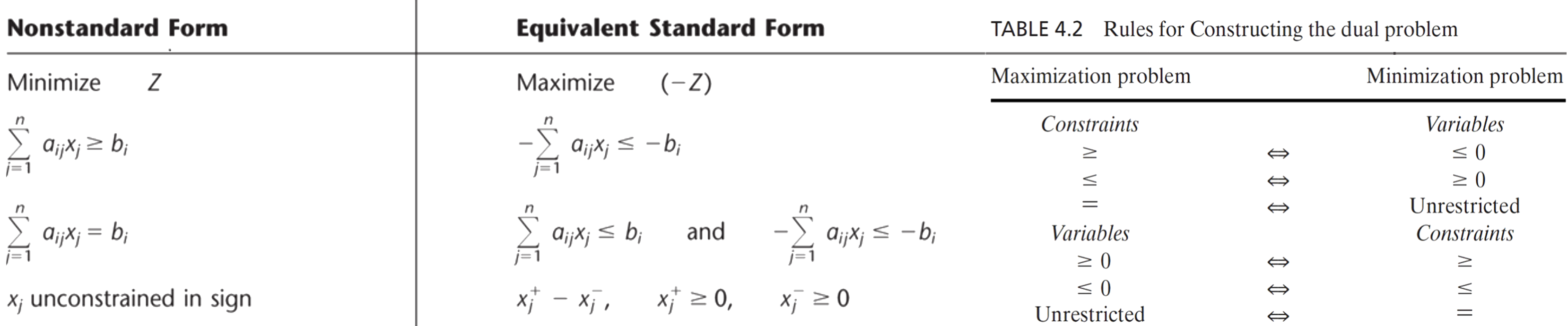
-
Example:
Use the primal-dual rules to determine the dual of the following model$$ \begin{aligned} & \text{min }Z=3x_2+x_3\\ & \text{s.t.} \begin{cases} & 3x_1 &- 5x_2 &- 7x_3 &+ x_4 &- x_5 &\le 0\\ & & 2x_2 &- x_3 &- 6x_4 &- 2x_5 &= 0\\ &-3x_1 &+ 2x_2 &- x_3 &- 4x_4 & &\le -7\\ & x_1 &+ x_2 &+ x_3 &+ x_4 & &\ge 12\\ & -x_1 &- x_2 &- x_3 &- 4x_4 & &\le 4\\ & x_1\ge 0, & x_2\ge 0, & x_4\ge 0, & x_5\ge 0 \end{cases} \end{aligned} $$transform into matrix form:
$\text{max }Z=3x_2+x_3$,$$ A= \begin{bmatrix} 3 & -5 & -7 & 1 & -1 \\ 0 & 2 & -1 & -6 & -2 \\ -3 & 2 & -1 & -4 & 0 \\ 1 & 1 & 1 & 1 & 0 \\ -1 & -1 & -1 & -4 & 0 \end{bmatrix}, b= \begin{bmatrix} 0\\ 0\\ -7\\ 12\\ 4 \end{bmatrix} $$where we have variables
$x_1,x_2,x_4,x_5\ge 0$and thus we have dual as given by:
$\text{min }b^Ty=-7y_3+12y_4+4y_5$,$$ A^T= \begin{bmatrix} 3 & 0 & -3 & -1 & -1\\ -5 & 2 & 2 & -1 & -1\\ -7 & -1 & -1 & -1 & -1\\ 1 & -6 & -4 & -1 & -4\\ -1 & -2 & 0 & 0 & 0 \end{bmatrix}, c= \begin{bmatrix} 0\\ 3\\ 1\\ 0\\ 0 \end{bmatrix} $$where by referring to Table 4.2 we have variables
$y_1,y_3,y_5\le 0,y_2\text{ unrestricted},y_4\ge 0$so in equation form we have
$$ \begin{aligned} &\text{max }-7y_3+12y_4+4y_5\\ &\text{s.t.} \begin{cases} 3y_1 & & & - & 3y_3 & - & y_4 & - & y_5 & \le & 0\\ -5y_1 & + & 2y_2 & + & 2y_3 & - & y_4 & - & y_5 & = & 3\\ -7y_1 & - & y_2 & - & y_3 & - & y_4 & - & y_5 & \le & 1\\ y_1 & - & 6y_2 & - & 4y_3 & - & y_4 & - & 4y_5 & \ge & 0\\ -y_1 & - & 2y_2 & & & & & & & \le & 0\\ y_1,y_3,y_5\le 0,&y_2\text{ unrestricted},&y_4\ge 0 \end{cases} \end{aligned} $$
Economic Interpretation
Consider the primal problem as being a resource allocation problem, e.g. we are trying to make products $x_1$, $x_2$, … Each product $j$ requires a certain amount $a_{ij}$ of each resource $i$ (like labour of machine time). Profits are $c_j$ for product $x_j$, and the object is to maximize total profits $c^Tx$. Now, assume we have $m$ kinds of resouces in total, and $n$ kinds of products. The equation form is given by
Now suppose we have an optimal solution $x^{\ast}$ to the primal problem.
- Due to strong duality we know there is a solution for the dual problem such that
$Z=c^Tx^{\ast}=b^Ty^{\ast}=W$. Where$b_i$represents the available amount of resource$i$in our resource allocation problem, and$y_i$is the contribution to profit (value) of having one unit of resource$i$. In this way$y_i$is called the dual price or shadow price of resource$i$. - When
$Z<W$, we have not reached an optimum, which economically can be interpreted that when revenues ($Z$) are less than the value of resources ($W$), we can always find a way to better exploit the resource.
Now reconsider this in matrix notation
when we replace $c_B^TB^{-1}$ by $y^{T}$, we shall find
with corresponding optimal value $Z^{\ast}=y^{\ast T}b$. So, with $b_i$ increase by 1, we now have $Z$ increased by $y_i^{\ast}$, and thus each entry $y_i$ in vector $y^{\ast T}=c_B^TB^{-1}$ is a shadow price!
Transportation Problem
-
Description
简单的说, 就是给定$m$个供应商,$n$个客户, 分别对应供应量与需求量, 现在给你运输成本$c_{ij}$, 让你求怎么供应成本最低. -
Model
令$x_{ij}$为供应量. LP如下$$ \begin{aligned} & \min Z=\sum_{i=1}^m\sum_{j=1}^nc_{ij}x_{ij}\\ & \text{ s.t.} \begin{cases} \sum_{j=1}^nx_{ij}=s_i\\ \sum_{i=1}^mx_{ij}=d_j\\ x_{ij}\ge 0 \end{cases} \end{aligned} $$当出现供应量总额与需求量总额不对等时, 引入dummies.
Transportation Simplex Method
Just some matrices.
Assignment Problem
-
Description
简单的说, 就是给你$n$个员工,$n$个活儿, 每个人只能干一个活并且不同组合工资$c_{ij}$各不一样, 现在问老板你怎么组合员工和工作, 付工资最少. -
Model
令二态变量$x_{ij}$为员工干/不干某个活儿. LP如下$$ \begin{aligned} & \min Z=\sum_{i=1}^m\sum_{j=1}^nc_{ij}x_{ij}\\ & \text{ s.t.} \begin{cases} \sum_{j=1}^nx_{ij}=1\\ \sum_{i=1}^mx_{ij}=1\\ x_{ij}\in\{0,1\} \end{cases} \end{aligned} $$类似的, 如果不对等, 就加入dummies.
Some Modeling Issues
-
或门/条件门
$$ \begin{aligned} & f_1(x)\le b_1+Mz\\ & f_2(x)\le b_2+M(1-z)\\ & z\in\{0,1\},\ M\text{ large} \end{aligned} $$ -
$N$选$K$$$ \begin{aligned} & f_k(x)\le b_k+Mz_k,\quad k=1,2,\ldots,N\\ & \sum_{k=1}^Nz_k=N-K\\ & z_k\in\{0,1\},\ M\text{ large} \end{aligned} $$ -
绝对值
-
出现在目标函数中: 令
$$ x=x^+-x^-,\quad x^+,x^-\ge 0 $$
则
$$ |x|=|x^+|+|x^-|. $$
仅在最小值问题中, 这样的绝对值替换是有效的.
-
出现在条件中
- 有界: 转化为同时成立问题.
- 无界: 转化为或门.
- 最大最小值/最小最大值问题 引入一个新变量, 替换掉嵌套在最值函数里面的那个最值, 并在条件中反映.
- Example: Faculty layout problem.
Max-flow/Min-cut Problem
-
Introduction
- Undirected/directed graphs
- Degree of a vertex/node
- Complete graphs
- Cost and capacities
- Walks, paths (walks without repeated vertices) and cycles (walks end at start)
- Cyclic/acyclic and forests
- (Strongly) connected graphs
- Bipartite graphs
-
Arc routing/Chinese Postman Problem 边的遍历/中国邮递员问题
- 如何遍历所有边并保证总权重最小. 令
$x_{ij}$为边$(i,j)$被走过的次数. ILP如下
$$ \begin{aligned} & \min\sum_{i=1}^n\sum_{j=1}^n c_{ij}x_{ij}\\ & \text{ s.t.} \sum_{j=1}^nx_{ij}-\sum_{j=1}^nx_{ji}=0\quad\text{for all }i=1,2,\ldots,n\\ & \qquad x_{ij}\ge 0\quad\text{for all }(i,j)\in A \end{aligned} $$- Euler cycle: 所有节点的度均为偶数, 则无向图有欧拉环
- Euler path: 只有0或者2个节点的度为奇数, 则无向图有欧拉路径
- 如何遍历所有边并保证总权重最小. 令
-
Minimal Spanning Tree 最小生成树
- 求一张图的最小权重生成树.
- NB: 一张有
$n$个节点的完全图有$n^{n-2}$棵生成树. - 算法:
- 随便挑一个点
- 贪心加陌生点
- 加完结束
-
Cuts 割
- 定义: A cut in a graph is a partition of the vertices into two disjoint sets.
- 性质: Given any cut in a graph, every minimal crossing edge belongs to some MST of the graph, and every MST contains a minimal crossing edge on the cut.
-
Shortest-route Problem 最短路径问题
- 与中国邮递员的不同: 不需要经过所有边(或者节点), 目标是从起点到终点
- Dijkstra算法: 不断更新节点的标签
$[u_j,i]=[u_i+d_{ij},i]$直到全部标签再也不变化.
-
Maximal Flow Algorithm 最大流问题
- 找出最大的总流量
- 算法: 不断更新标签
$[c_{ik},k]$直到所有标签不再变化. 其中$c_{ik}=\max_{j\in S_i}\{c_{ij}\}$. - ILP for the maximal flow problem
-
Minimal Cut Problem 最小割问题
就是找出最小总权值的割, 与最大流问题是等价的. -
Max-flow/min-cut theorem 最大流最小割定理
在任何一张网络中, 最大流恒等价于最小割.
Heuristics
贪心、局部搜索、Tabu搜索、模拟退火、神经网络… 略. 基本不会考.
Dynamic Programming (DP)
-
Decision tree 决策树
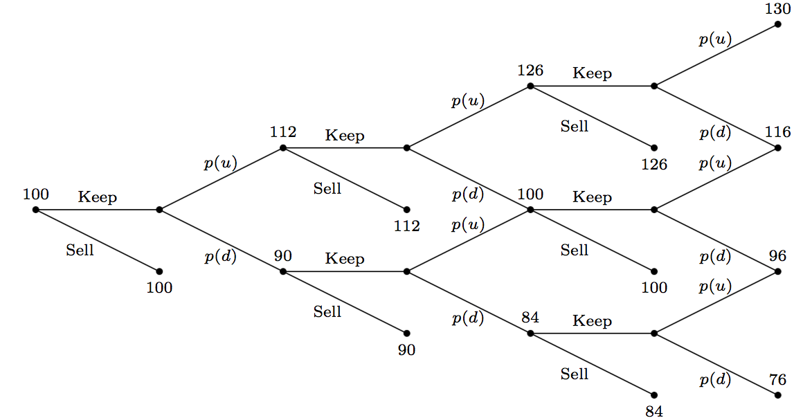
自后向前优化的一个过程. 这就是逆序动态规划.
-
General dynamic programming 一般动态规划
- Process:
- Devide a problem into stages.
- Solve from the very last stage, say,
$n$. - Use the optimum of stage
$n$to solve the optimization problem of state$n-1$, etc.
- Bellman equation 贝尔曼方程:
$$ f_i(s_i)=\min_{x_i}{c(s_i,x_i)+f_{i+1}(s_{i+1})}. $$
In stochastic dynamic programming, the state after decision is random and thus we have the Bellman equation instead as
$$ f_i(s_i)=\min_{x_i}{c(s_i,x_i)+\text{E}[f_{i+1}(s_{i+1})]}. $$
- NB: There could be overlapping subproblems, see node with weight 116 on the upper right of the figure above.
-
Examples
- Project investment
- Hiring job candidates
- Shortest-route problem
- Workforce planning
- Solving LP’s using dynamic programming (treat the variables as stages)
- Ordering inventory (simplifies to never order in periods where we still have inventory)
- Egg-breaking (
$n$eggs,$k$floors, Bellman$f(n,k)=1+\min_x\max\{f(n-1,x-1),f(n,k-x)\}$, deciding the floor for the first trial,$x$.)
Traveling Salesman Problem (TSP)
-
Description
推销员要去所有城市(恰好一次), 并且希望总路程最短且最后能回来. -
Algorithm complexity: example of shortest-route algorithm 以最短路径问题为例
- 第一次迭代时需要计算
$u_j=\min\{u_j,u_i+d_{ij}\}$, 即$n-1$次加法与$n-1$次比较, 另加上最后从所有$u_j$中挑出最小的一个, 又是$n-1$次比较. - 故第一次迭代共
$3n-3$次运算. - 类推, 时间复杂度为
$O[3n(n-1)/2]=O(n^2)$. - 然后考虑推销员问题, 我们会发现无论如何不能由多项式表示其复杂度, 因而把它归类为NP-hard问题, 即在多项式时间内可以转化为NP-complete的问题.
- 但NP-complete暂时归为NP, 即多项式内不可解. 因为我们无法写出其多项式表达式.
- 第一次迭代时需要计算
-
Graph 图
- Cycle 环: start=end
- Hamiltonian cycle 哈密尔顿环: 包含每个节点恰好一次的环
- 因此: 推销员问题亦即是最小哈密尔顿环问题.
-
ILP 如下
$$ \begin{aligned} & \min\sum_{i=1}^n\sum_{j=1}^n c_{ij}x_{ij}\\ & \text{ s.t.} \begin{cases} \sum_{j=1}^nx_{ij}=1,\quad i=1,2,\ldots,n\\ \sum_{i=1}^nx_{ij}=1,\quad j=1,2,\ldots,n\\ x_{ij}\in\{0,1\}. \end{cases} \end{aligned} $$这不就是assignment problem 运输问题嘛!
当然是有区别的, 不然就不会分开教了. 其实上面的ILP完全就是分工问题, 而推销员问题还要加上没有subtour 子环游这个条件:$$ (1)\ \sum_{i\in S}\sum_{j\in S}x_{ij}\le |S|-1\qquad (2)\ \sum_{i\in S}\sum_{j\in\bar S}x_{ij}\ge 1\qquad (3)\ u_i-u_j+nx_{ij}\le n-1,\ \forall i,j $$
任选其一. 其中
$S\subset N$,$N$为所有节点的集合. 直白地讲, 就是随便画个圈, 不可能把这个tour给分成两部分, 必定有边被切断. -
估计时间复杂度的范围
- 虽然是
$NP-hard$的, 我们仍然可以把推销员问题与别的$P$问题(什么地方怪怪的)做比较, 从而得到它的时间复杂度的范围. 一个很容易想到的例子就是上面提到的分工问题. 分工问题的条件比推销员问题松, 所以推销员问题的解必定是分工问题的解, 但反之不成立. 这说明分工问题给出了复杂度的一个下界. - 另一方面, 考虑到如果从推销员问题的解中删除一条边, 我们就会得到一棵生成树, 所以最小生成树算法也给出了一个下界.
- 虽然是
-
具体算法
- Iteration: 从分工问题中找推销员问题的解, 逐渐增加条件
- Dynamic programming: 从两个城市开始考虑, 逐渐增加城市个数, 最后考虑节点全集. 考虑的情况有
$2^n$种, 每种最多包含$n$个节点(包括起点$1$), 令任意一个节点为终点, 都有至少$n$条最短路径. 因而时间复杂度为$O(n^22^n)$. - Heuristics: 包括
- Nearest Neighbor 近邻算法 (
$NN(I)\ge rOPT(I)$), - MST 最小生成树算法 (
$MST(I)\le 2OPT(I)$), - Cheapest Insertion 廉价插入算法 (
$CI(I)\le 2OPT(I)$).
- Nearest Neighbor 近邻算法 (