LDA and R-MDA
2018-05-29
This is a note of Linear Discriminant Analysis (LDA) and an original Regularized Matrix Discriminant Analysis (R-MDA) method proposed by Jie Su et al, 2018. Both methods are suitable for efficient multiclass classification, while the latter is a state-of-the-art version of the classical LDA method s.t. data in matrix forms can be classified without destroying the original structure.
A Sketch of LDA
The plain idea behind Discriminant Analysis is to find the optimal partition (or projection, for higher-dimensional problems) s.t. entities within the same class are distributed as compactly as possible and entities between classes are distributed as sparsely as possible. To derive closed-form solutions we have various conditions on the covariance matrices of the input data. When we assume covariances $\boldsymbol{\Sigma}_k$ are equal for all classes $k\in\{1,2,\ldots,K\}$, we’re following the framework of Linear Discriminant Analysis (LDA).
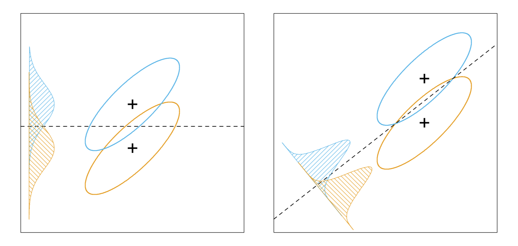
As shown above, when we consider a 2-dimensional binary classification problem, the LDA is equivalently finding the optimal direction vector $\mathbf{w}$ s.t. the ratio of $\mathbf{w}^T\mathbf{S}_b\mathbf{w}$ (sum of between-class covariances of the projections) and $\mathbf{w}^T\mathbf{S}_w\mathbf{w}$ (sum of within-class covariances of the projections) is maximized. Specifically, we define
$$ \mathbf{S}_b = (\boldsymbol{\mu}_0 - \boldsymbol{\mu}_1)^T(\boldsymbol{\mu}_0 - \boldsymbol{\mu}_1) $$
and
Therefore, the objective of this maximization problem is
$$ J = \frac{\mathbf{w}^T\mathbf{S}_b\mathbf{w}}{\mathbf{w}^T\mathbf{S}_w\mathbf{w}} $$
which is also called the generalized Rayleigh quotiet.
The homogenous objective can be equivalently written into
$$ \begin{align} \min_{\mathbf{w}}\quad &-\mathbf{w}^T\mathbf{S}_b\mathbf{w}\\ \text{s.t.}\quad &\mathbf{w}^T\mathbf{S}_w\mathbf{w} = 1 \end{align} $$
which, by using the method of Langrange multipliers, gives solution
$$ \mathbf{w} = \mathbf{S}_w^{-1}(\boldsymbol{\mu}_0 - \boldsymbol{\mu}_1) $$
and the final prediction for new data $\mathbf{x}$ is based on the scale of $\mathbf{w}^T\mathbf{x}$.
For multiclass classification, the solution is similar. Here we propose the score function below without derivation:
$$ \delta_k = \mathbf{x}^T\boldsymbol{\Sigma}^{-1}\boldsymbol{\mu}_k - \frac{1}{2}\boldsymbol{\mu}_k^T\boldsymbol{\Sigma}^{-1}\boldsymbol{\mu}_k + \log\pi_k $$
where $\boldsymbol{\mu}_k$ is the sample mean of all data within class $k$, and $\pi_k$ is the percentage of all data that is of this class. By comparing these $k$ scores we determine the best prediction with the highest value.
Codes of LDA
We first load necessary packages.
%config InlineBackend.figure_format = 'retina'

import warnings
import numpy as np
import matplotlib.pyplot as plt
from matplotlib import rcParams, rc
from scipy.optimize import minimize

warnings.simplefilter('ignore')
rcParams['pdf.fonttype'] = 42
rc("font", **{'family': 'serif', 'serif': ['Palatino'], 'size':13})
rc("text", usetex = True)
rc('legend', **{'frameon': False, 'loc': 'upper right', 'fontsize': 15})
colors = ['#b80b0b', '#b89a0b', '#378000', '#2e157e']
Now we define a new class called LDA with a predict (in fact also predict_prob) method.
class LDA:
    def __init__(self, X, y):  # X is 2D, y is 1D
        assert len(X) == len(y), 'X and y should have the same lengths.'
        n_features = len(X[0])
        classes = list(set(y))
        labels = {c: [] for c in classes}
        for _X, _y in zip(X, y):
            labels[_y].append(_X)
        labels = {c: np.array(labels[c]).reshape(-1, n_features) \
                  for c in classes}
        pi = {c: len(labels[c]) for c in classes}
        mu = {c: labels[c].sum(axis=0) / pi[c] for c in classes}
        Sigma = sum(np.cov(labels[c], rowvar=False) for c in classes)
        inv_Sigma = np.linalg.inv(Sigma)
        self.predict_prob = lambda x: {c: np.array(x) @ inv_Sigma @ mu[c].T - \
                                          mu[c] @ inv_Sigma @ mu[c].T / 2 + \
                                          np.log(pi[c])
                                       for c in classes}

    def predict(self, x):
        prob = self.predict_prob(x)
        return max(prob, key=prob.get)
Then we define three classes of 2D input $\mathbf{X}$ and pass it to the classifier. Original as well as the predicted distributions are plotted with accuracy printed below.
np.random.seed(2)

N = 100
X = np.vstack([np.random.normal(loc=(0,10), scale=5, size=(N,2)),
               np.random.normal(loc=(10,-8), scale=5, size=(N,2)),
               np.random.normal(loc=(-10,-8), scale=5, size=(N,2))])
y = [0] * N + [1] * N + [2] * N

fig = plt.figure(figsize=(14, 7))

ax = fig.add_subplot(121)
for _X, _y in zip(X, y):
    ax.scatter(_X[0], _X[1], c=colors[_y], s=50,
               alpha=.5, edgecolor='none')
ax.set_xlim(-25, 25)
ax.set_ylim(-25, 25)
ax.set_title('Original Classes')

cls = LDA(X, y)

ax = fig.add_subplot(122)
correct = 0
for _X, _y in zip(X, y):
    _y_pred = cls.predict(_X)
    correct += (_y == _y_pred)
    ax.scatter(_X[0], _X[1], c=colors[_y_pred], s=50,
               alpha=.5, edgecolor='none')
ax.set_xlim(-25, 25)
ax.set_ylim(-25, 25)
ax.set_title('Predicted Classes')

plt.show()

accuracy = correct / (3 * N)
print('Training accuracy: {:.2f}%'.format(accuracy * N))
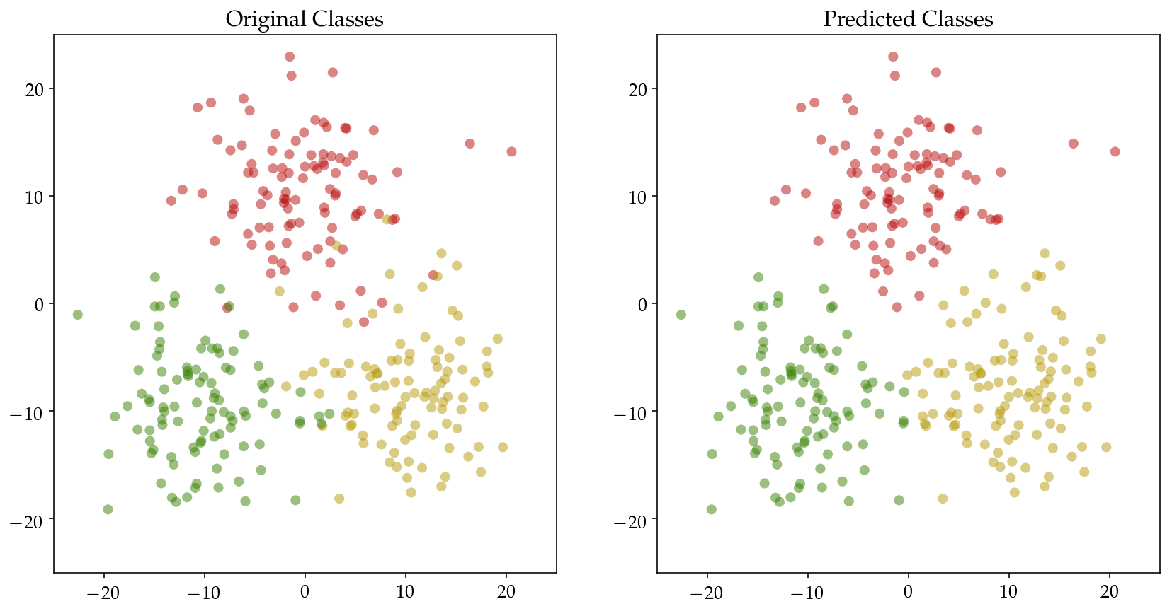
Training accuracy: 95.67%
A Sketch of R-MDA
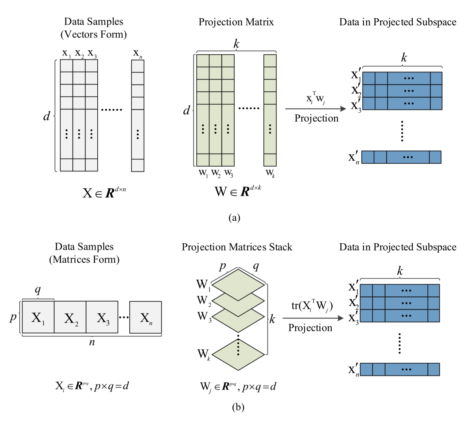
For data with inherent matrix forms like electroencephalogram (EEG) data introduced in Jie Su (2018), the classical LDA is not the most appropriate solution since it forcibly requires vector input. To use LDA for classification on such datasets we have to vectorize the matrices and potentially losing some critical structural information. Authors of this paper invented this new method called Regularized Matrix Discriminant Analysis (R-MDA) that naturally takes matric input in analysis. Furthermore, noticing that inversing large matrix $\mathbf{S}_w$ in high dimensions can be computationally burdonsome, they adopted the Alternating Direction Method of Multipliers (ADMM) to iteratively optimize the objective instead of the widely-used Singular Valur Decomposition (SVD). A graphical representation of the R-MDA compared with LDA is as follows.
The algorithm is implemented below. Notice here I skipped the Gradient Descent (GD) approach in the minimization during iterations and opt for the minimize function in scipy.optimize. I did so to make the structure simpler without hurting the understanding of the whole algorithm. For more detailed illustration please resort to the original paper.
Codes of R-MDA
Again we first define the class RMDA. The predict method now takes a matrix.
class RMDA:
    def __init__(self, X, y, learning_rate=0.01, max_iter=100, tau=0.05, rho=0.01):  # X is 3D, y is 1D
        assert len(X) == len(y), 'X and y should have the same lengths.'
        shape = X[0].shape
        classes = list(set(y))
        labels = {c: [] for c in classes}
        for _X, _y in zip(X, y):
            labels[_y].append(_X)
        n = {c: len(labels[c]) for c in classes}
        N = len(y)
        K=  len(classes)
        mu = sum(X) / N
        X_tilde = [_X - mu for _X in X]
        Y_tilde = np.zeros((N, K))
        for i in range(N):
            for j in range(K):
                if y[i] == classes[j]:
                    Y_tilde[i,j] = np.sqrt(N / n[j]) - np.sqrt(n[j] / N)
                else:
                    Y_tilde[i,j] = -np.sqrt(n[j] / N)
        W = [np.random.normal(size=shape[::-1]) for j in range(K)]
        L = lambda W: sum((np.trace(X_tilde[i].dot(W[j])) - Y_tilde[i,j])**2 \
                          for i in range(N) for j in range(K)) / (2 * N) + \
                      sum(self.nuclear_norm(W[j]) for j in range(K)) * tau
        S = [np.random.normal(size=shape) for j in range(K)]
        V = [np.random.normal(size=shape) for j in range(K)]
        L_temp = 0
        for iteration in range(max_iter):
            for j in range(K):
                L1 = lambda w: sum((np.trace(X_tilde[i].dot(w)) - Y_tilde[i,j])**2 \
                                   for i in range(N)) / (2 * N) - \
                               np.trace(V[j].dot(w)) + \
                               self.frobenius_norm(S[j] - w)**2 * rho / 2
                L1_ = lambda w: L1(w.reshape(shape))
                W[j] = minimize(fun=L1_, x0=W[j]).x.reshape(shape)
                L2 = lambda s: self.nuclear_norm(s) * tau + \
                               np.trace(V[j].dot(s)) + \
                               self.frobenius_norm(S[j] - w)**2 * rho / 2
                L2_ = lambda s: L2(s.reshape(shape))
                S[j] = minimize(fun=L2_, x0=S[j]).x.reshape(shape)
                V[j] -= (W[j] - S[j]) * rho
            L_W = L(W)
            dL = abs(L_W - L_temp)
            print('[{}/{}] {:<10.4f}'.format(iteration + 1, max_iter, dL), end='\r')
            L_temp = L_W
            if dL < 1e-9: break
        if iteration == max_iter - 1:
            print('Optimization failed to converge.')
        else:
            print('Optimization converged successfully.')
        self.predict_prob = lambda X: {classes[j]: np.trace(X.dot(W[j])) for j in range(K)}

    def nuclear_norm(self, X):
        return np.linalg.svd(X)[1].sum()

    def frobenius_norm(self, X):
        return sum(X[i,j]**2 for i in range(X.shape[0]) for j in range(X.shape[1]))

    def predict(self, X):
        prob = self.predict_prob(X)
        return max(prob, key=prob.get)
Then we train the model and print the final accuracy.
np.random.seed(2)

N = 100
X = np.vstack([np.random.normal(loc=((10,0),(0,10)), scale=5, size=(N,2,2))] + \
              [np.random.normal(loc=((0,10),(10,0)), scale=5, size=(N,2,2))] + \
              [np.random.normal(loc=((-8,-8),(-8,8)), scale=5, size=(N,2,2))])
y = [0] * N + [1] * N + [2] * N

cls = RMDA(X, y)
correct = 0
for _X, _y in zip(X, y):
    _y_pred = cls.predict(_X)
    correct += (_y == _y_pred)

accuracy = correct / (3 * N)
print('Training accuracy: {:.2f}%'.format(accuracy * 100))
Optimization converged successfully.
Training accuracy: 87.00%
Further analysis and debugging should be expected. Any correction in comments is also welcomed. 😇
References
- Su, Jie, Linbo Qing, Xiaohai He, Hang Zhang, Jing Zhou, and Yonghong Peng. “A New Regularized Matrix Discriminant Analysis (R-MDA) Enabled Human-Centered EEG Monitoring Systems.” IEEE Access 6 (2018): 13911-13920.
- Friedman, Jerome, Trevor Hastie, and Robert Tibshirani. The elements of statistical learning. Vol. 1. New York: Springer series in statistics, 2001.