Literature Review on Optimal Order Execution (5)
2018-05-12
This is the fifth post on optimal order execution. Based on Almgren and Chriss (2000), today we attempt to estimate the market impact coefficient $\eta$. Specifically, for high-frequency transaction data, we have the approximation $dS = \eta\cdot dQ$ and thus can easily estimate it by the method of Ordinary Least Squares (OLS), using the message book data provided by LOBSTER.
Experiment: Apple
We first explore the message book of Apple Inc. (symbol: AAPL) from 09:30 to 16:00 on June 21, 2012.
import pandas as pd
import numpy as np
import statsmodels.formula.api as sm
import matplotlib.pyplot as plt
pd.options.mode.chained_assignment = None
According to the instructions by LOBSTER, the columns of the message book are defined as follows:
- time: seconds after midnight with decimal precision of at least milliseconds and up to nanoseconds depending on the requested period
- type:
1means submission of a new limit order;2means Cancellation (partial deletion of a limit order);3means deletion (total deletion of a limit order);4means execution a visible limit order;5means Execution of a hidden limit order;7means Trading halt indicator (detailed information below) - id: unique order reference number (assigned in order flow)
- size: number of shares
- price: dollar price times 10000 (i.e., a stock price of 91.14USD is given by 911400)
- direction:
-1means means Sell limit order;1means Buy limit order
message = pd.read_csv('data/AAPL_2012-06-21_34200000_57600000_message_1.csv', header=None)
message.columns = ['time', 'type', 'id', 'size', 'price', 'direction']
message.price /= 10000
message.head()
| time | type | id | size | price | direction | |
|---|---|---|---|---|---|---|
| 0 | 34200.004241 | 1 | 16113575 | 18 | 585.33 | 1 |
| 1 | 34200.025552 | 1 | 16120456 | 18 | 585.91 | -1 |
| 2 | 34200.201743 | 3 | 16120456 | 18 | 585.91 | -1 |
| 3 | 34200.201781 | 3 | 16120480 | 18 | 585.92 | -1 |
| 4 | 34200.205573 | 1 | 16167159 | 18 | 585.36 | 1 |
| 5 | 34200.201781 | 3 | 16120480 | 18 | 585.92 | -1 |
| 6 | 34200.205573 | 1 | 16167159 | 18 | 585.36 | 1 |
message_plce = message[message.type==1]
message_exec = message[message.type==4]
message_temp = pd.merge(message_plce, message_exec, on='id', how='inner')
message_temp.columns
Index(['time_x', 'type_x', 'id', 'size_x', 'price_x', 'direction_x', 'time_y',
       'type_y', 'size_y', 'price_y', 'direction_y'],
      dtype='object')
df = message_temp[['id', 'time_x', 'time_y', 'size_y', 'price_x', 'direction_x']]
df.columns = ['id', 'ts', 'te', 'size', 'price', 'direction']
df['duration'] = df.te - df.ts
df.shape
(15099, 7)
Here I defined a function impact to calculate the market impact (reflected on price deviation), such that for each successful execution, we calculate the price change after the same duration of the order.
def impact(idx):
    S0, t, duration = df.loc[idx, ['price', 'te', 'duration']]
    i = None
    for i in range(message_exec[message_exec.time==t].index[0], len(message_exec)):
        try:
            T = message_exec.loc[i, 'time']
            ST = message_exec.loc[i, 'price']
            if T - t >= duration: break
        except:
            pass
    if not i: return np.nan
    return ST - S0
df['impact'] = [impact(i) for i in df.index]

df_reg = df.dropna()[['size', 'impact']]
df_reg.columns = ['dQ', 'dS']
df_reg.dS = df_reg.dS.abs()
df_reg.T
| 0 | 1 | 2 | 3 | 4 | 5 | 6 | … | 2456 | 2457 | 2458 | 2459 | 2460 | 2461 | |
|---|---|---|---|---|---|---|---|---|---|---|---|---|---|---|
| dQ | 1.0 | 10.0 | 9.00 | 40.00 | 18.00 | 100.00 | 18.00 | … | 10.00 | 40.00 | 50.00 | 1.00 | 100.00 | 100.00 |
| dS | 0.2 | 0.2 | 0.03 | 0.19 | 0.07 | 0.09 | 0.21 | … | 0.05 | 0.05 | 0.05 | 0.08 | 0.08 | 0.03 |
fig = plt.figure(figsize=(14, 6))
ax = fig.add_subplot(111)
ax.scatter(df_reg.dQ, df_reg.dS, color='k', s=2)
ax.set_xlabel('dQ')
ax.set_ylabel('dS')
plt.tight_layout()
plt.show()
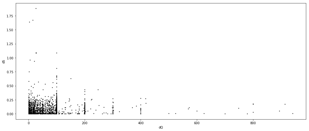
res = sm.ols(formula='dS ~ dQ + 0', data=df_reg).fit()
print(res.summary())
                            OLS Regression Results
==============================================================================
Dep. Variable:                     dS   R-squared:                       0.148
Model:                            OLS   Adj. R-squared:                  0.148
Method:                 Least Squares   F-statistic:                     427.7
Date:                Sat, 12 May 2018   Prob (F-statistic):           1.01e-87
Time:                        14:02:16   Log-Likelihood:                 1535.7
No. Observations:                2459   AIC:                            -3069.
Df Residuals:                    2458   BIC:                            -3064.
Df Model:                           1
Covariance Type:            nonrobust
==============================================================================
                 coef    std err          t      P>|t|      [0.025      0.975]
------------------------------------------------------------------------------
dQ             0.0005   2.37e-05     20.680      0.000       0.000       0.001
==============================================================================
Omnibus:                     2646.045   Durbin-Watson:                   1.287
Prob(Omnibus):                  0.000   Jarque-Bera (JB):           323199.873
Skew:                           5.154   Prob(JB):                         0.00
Kurtosis:                      58.210   Cond. No.                         1.00
==============================================================================

Warnings:
[1] Standard Errors assume that the covariance matrix of the errors is correctly specified.
Apparently there’re several outliers that result in a low $R^2$. Here we remove outliers that are lying outside three standard deviations.
df_reg_no = df_reg[((df_reg.dQ - df_reg.dQ.mean()).abs() < df_reg.dQ.std() * 3) &
                   ((df_reg.dS - df_reg.dS.mean()).abs() < df_reg.dS.std() * 3)]
fig = plt.figure(figsize=(14, 6))
ax = fig.add_subplot(111)
ax.scatter(df_reg_no.dQ, df_reg_no.dS, color='k', s=2)
ax.set_xlabel('dQ')
ax.set_ylabel('dS')
plt.tight_layout()
plt.show()
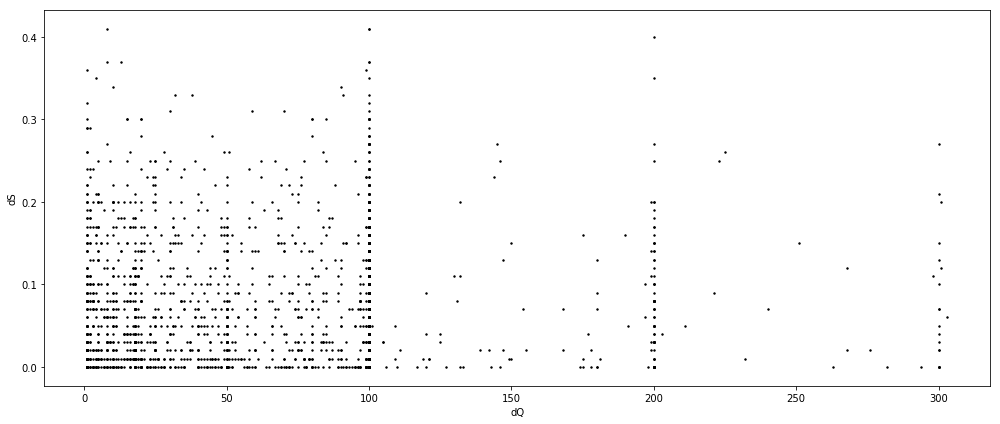
res = sm.ols(formula='dS ~ dQ + 0', data=df_reg_no).fit()
print(res.summary())
                            OLS Regression Results
==============================================================================
Dep. Variable:                     dS   R-squared:                       0.296
Model:                            OLS   Adj. R-squared:                  0.295
Method:                 Least Squares   F-statistic:                     1005.
Date:                Sat, 12 May 2018   Prob (F-statistic):          1.45e-184
Time:                        14:02:20   Log-Likelihood:                 2470.2
No. Observations:                2397   AIC:                            -4938.
Df Residuals:                    2396   BIC:                            -4933.
Df Model:                           1
Covariance Type:            nonrobust
==============================================================================
                 coef    std err          t      P>|t|      [0.025      0.975]
------------------------------------------------------------------------------
dQ             0.0006   1.97e-05     31.710      0.000       0.001       0.001
==============================================================================
Omnibus:                      356.596   Durbin-Watson:                   1.108
Prob(Omnibus):                  0.000   Jarque-Bera (JB):              567.767
Skew:                           1.012   Prob(JB):                    5.14e-124
Kurtosis:                       4.259   Cond. No.                         1.00
==============================================================================

Warnings:
[1] Standard Errors assume that the covariance matrix of the errors is correctly specified.
So we conclude $\hat{\eta}_{\text{AAPL}}=0.0006$ for the underlying timespan. However, what about other companies? The coefficients are expected to vary largely, which is though the very worst case we’d like to see.
Comparison
We first define a function estimate to automate what we’ve done above.
def estimate(symbol):
    message = pd.read_csv('data/{}_2012-06-21_34200000_57600000_message_1.csv'.format(symbol), header=None)
    message.columns = ['time', 'type', 'id', 'size', 'price', 'direction']
    message.price /= 10000
    message_plce = message[message.type==1]
    message_exec = message[message.type==4]
    message_temp = pd.merge(message_plce, message_exec, on='id', how='inner')
    df = message_temp[['id', 'time_x', 'time_y', 'size_y', 'price_x', 'direction_x']]
    df.columns = ['id', 'ts', 'te', 'size', 'price', 'direction']
    df['duration'] = df.te - df.ts
    def impact(idx):
        S0, t, duration = df.loc[idx, ['price', 'te', 'duration']]
        i = None
        for i in range(message_exec[message_exec.time==t].index[0], len(message_exec)):
            try:
                T = message_exec.loc[i, 'time']
                ST = message_exec.loc[i, 'price']
                if T - t >= duration: break
            except:
                pass
        if not i: return np.nan
        return ST - S0
    df['impact'] = [impact(i) for i in df.index]
    df_reg = df.dropna()[['size', 'impact']]
    df_reg.columns = ['dQ', 'dS']
    df_reg.dS = df_reg.dS.abs()
    df_reg_no = df_reg[((df_reg.dQ - df_reg.dQ.mean()).abs() < df_reg.dQ.std() * 3) &
                       ((df_reg.dS - df_reg.dS.mean()).abs() < df_reg.dS.std() * 3)]
    res = sm.ols(formula='dS ~ dQ + 0', data=df_reg_no).fit()
    print(res.summary())
The estimation for Microsoft Corp. (symbol: MSFT) is as follows.
estimate('MSFT')
                            OLS Regression Results
==============================================================================
Dep. Variable:                     dS   R-squared:                       0.229
Model:                            OLS   Adj. R-squared:                  0.228
Method:                 Least Squares   F-statistic:                     550.7
Date:                Sat, 12 May 2018   Prob (F-statistic):          7.20e-107
Time:                        14:04:51   Log-Likelihood:                 5732.8
No. Observations:                1859   AIC:                        -1.146e+04
Df Residuals:                    1858   BIC:                        -1.146e+04
Df Model:                           1
Covariance Type:            nonrobust
==============================================================================
                 coef    std err          t      P>|t|      [0.025      0.975]
------------------------------------------------------------------------------
dQ          1.859e-05   7.92e-07     23.467      0.000     1.7e-05    2.01e-05
==============================================================================
Omnibus:                      201.842   Durbin-Watson:                   0.778
Prob(Omnibus):                  0.000   Jarque-Bera (JB):              381.770
Skew:                           0.703   Prob(JB):                     1.26e-83
Kurtosis:                       4.719   Cond. No.                         1.00
==============================================================================

Warnings:
[1] Standard Errors assume that the covariance matrix of the errors is correctly specified.
The estimation for Amazon.com, Inc. (symbol: AMZN) is as follows.
estimate('AMZN')
                            OLS Regression Results
==============================================================================
Dep. Variable:                     dS   R-squared:                       0.294
Model:                            OLS   Adj. R-squared:                  0.293
Method:                 Least Squares   F-statistic:                     328.9
Date:                Sat, 12 May 2018   Prob (F-statistic):           1.02e-61
Time:                        14:06:56   Log-Likelihood:                 809.19
No. Observations:                 791   AIC:                            -1616.
Df Residuals:                     790   BIC:                            -1612.
Df Model:                           1
Covariance Type:            nonrobust
==============================================================================
                 coef    std err          t      P>|t|      [0.025      0.975]
------------------------------------------------------------------------------
dQ             0.0007   3.74e-05     18.136      0.000       0.001       0.001
==============================================================================
Omnibus:                      141.501   Durbin-Watson:                   1.022
Prob(Omnibus):                  0.000   Jarque-Bera (JB):              250.801
Skew:                           1.083   Prob(JB):                     3.46e-55
Kurtosis:                       4.709   Cond. No.                         1.00
==============================================================================

Warnings:
[1] Standard Errors assume that the covariance matrix of the errors is correctly specified.
The estimation for Alphabet Inc. (symbol: GOOG) is as follows.
estimate('GOOG')
                            OLS Regression Results
==============================================================================
Dep. Variable:                     dS   R-squared:                       0.419
Model:                            OLS   Adj. R-squared:                  0.418
Method:                 Least Squares   F-statistic:                     324.2
Date:                Sat, 12 May 2018   Prob (F-statistic):           5.96e-55
Time:                        14:07:20   Log-Likelihood:                 169.55
No. Observations:                 450   AIC:                            -337.1
Df Residuals:                     449   BIC:                            -333.0
Df Model:                           1
Covariance Type:            nonrobust
==============================================================================
                 coef    std err          t      P>|t|      [0.025      0.975]
------------------------------------------------------------------------------
dQ             0.0017   9.57e-05     18.005      0.000       0.002       0.002
==============================================================================
Omnibus:                       48.913   Durbin-Watson:                   1.331
Prob(Omnibus):                  0.000   Jarque-Bera (JB):               61.896
Skew:                           0.864   Prob(JB):                     3.63e-14
Kurtosis:                       3.563   Cond. No.                         1.00
==============================================================================

Warnings:
[1] Standard Errors assume that the covariance matrix of the errors is correctly specified.
The estimation for Intel Corp. (symbol: INTC) is as follows.
estimate('INTC')
                            OLS Regression Results
==============================================================================
Dep. Variable:                     dS   R-squared:                       0.237
Model:                            OLS   Adj. R-squared:                  0.237
Method:                 Least Squares   F-statistic:                     444.2
Date:                Sat, 12 May 2018   Prob (F-statistic):           4.52e-86
Time:                        14:08:47   Log-Likelihood:                 4480.8
No. Observations:                1429   AIC:                            -8960.
Df Residuals:                    1428   BIC:                            -8954.
Df Model:                           1
Covariance Type:            nonrobust
==============================================================================
                 coef    std err          t      P>|t|      [0.025      0.975]
------------------------------------------------------------------------------
dQ          2.275e-05   1.08e-06     21.076      0.000    2.06e-05    2.49e-05
==============================================================================
Omnibus:                      164.136   Durbin-Watson:                   0.716
Prob(Omnibus):                  0.000   Jarque-Bera (JB):              284.351
Skew:                           0.762   Prob(JB):                     1.79e-62
Kurtosis:                       4.566   Cond. No.                         1.00
==============================================================================

Warnings:
[1] Standard Errors assume that the covariance matrix of the errors is correctly specified.
Conclusion
In sum, the market impact are generally significant but not leading to high $R^2$ values, which suggests the linear assumption might be too strong. Also, it is noteworthy that $\hat{\eta}$ does vary largely between companies (let alone industries or equity types), which means we cannot use one estimation as a benchmark for general production usage.