These are the notes taken on my master course Multivariate Data Analysis via Matrix Decomposition. If you’re confused with the course name, you can think of this as a statistical course on unsupervised learning. $\newcommand{1}[1]{\unicode{x1D7D9}_{\{#1\}}}\newcommand{Corr}{\text{Corr}}\newcommand{E}{\text{E}}\newcommand{Cov}{\text{Cov}}\newcommand{Var}{\text{Var}}\newcommand{span}{\text{span}}\newcommand{bs}{\boldsymbol}\newcommand{R}{\mathbb{R}}\newcommand{rank}{\text{rank}}\newcommand{\norm}[1]{\left\lVert#1\right\rVert}\newcommand{diag}{\text{diag}}\newcommand{tr}{\text{tr}}\newcommand{braket}[1]{\left\langle#1\right\rangle}\newcommand{C}{\mathbb{C}}$

Notations

First let’s give some standard notations used in this course. Let’s assume no prior knowledge in linear algebra and start from matrix multiplication.

Matrix Multiplication

We denote a matrix $\mathbf{A}\in\R^{m\times n}$, with its entries defined as $[a_{ij}]_{i,j=1}^{m,n}$. Similarly, we define $\mathbf{B}=[b_{jk}]_{j,k=1}^{n,p}$ and thus the multiplication is defined as $\mathbf{AB} = [\sum_{j=1}^n a_{ij}b_{jk}]_{i,k=1}^{n,p}$, which can also be represented in three other ways:

• vector form, using $\mathbf{a}$ and $\mathbf{b}$
• a matrix of products of $A$ and $\mathbf{b}$
• a matrix of products of $\mathbf{a}$ and $\mathbf{B}$

A special example of such representation: let’s assume

$$ \mathbf{A}=[\mathbf{a}_1,\mathbf{a}_2,\ldots,\mathbf{a}_n]\in\R^{m\times n}\text{ and } \mathbf{D} = \diag(d_1,d_2,\ldots,d_n) \in\R^{n\times n},$$

then we have right away $\mathbf{AD}=[\mathbf{a}_id_i]_{i=1}^n$.

Exercise With multiplication we care ranks of matrices. There is a quick conclusion: If $\mathbf{x}\neq \bs{0}, \mathbf{y}\neq \bs{0}$, then $\rank(\bs{yx'})=1$. Conversely, if $\rank(\mathbf{A})=1$, then $\exists\ \mathbf{x}\neq \bs{0}, \mathbf{y}\neq \bs{0}$ s.t. $\bs{xy'}=\mathbf{A}$. Prove it.

Norms

There are two types of norms in this course we consider:

• (Euclidean) We define the $l^1$-norm as $\norm{\mathbf{x}}_1 = \sum_{i=1}^n |x_i|$, define $l^2$-norm as $\norm{\mathbf{x}}_2 = \sqrt{\mathbf{x'x}}$, define $l^{\infty}$-norm as $\norm{\mathbf{x}}_{\infty} = \max_{1\le i \le n}\{|x_i|\}$, and define the Mahalanobis norm as $\norm{\mathbf{x}}_A = \sqrt{\mathbf{x'Ax}}$.
• (Frobenius) We define the Frobenius norm of a matrix as $\norm{\mathbf{A}}_F=\sqrt{\sum_{i=1}^m\sum_{j=1}^n a_{ij}^2}$. The spectral 2-norm of a matrix is defined as $\norm{\mathbf{A}}_2=\max_{\mathbf{x}\neq \bs{0}} \norm{\mathbf{Ax}}_2 / \norm{\mathbf{x}}_2$.

Properties of these norms:

• $\norm{\mathbf{v}}=0$ iff. $\mathbf{v}=\bs{0}$.
• $\norm{\alpha \mathbf{v}} = |\alpha|\cdot\norm{\mathbf{v}}$ for any $\alpha\in\R$ and any $\mathbf{v}\in\mathcal{V}$.
• (Triangular Inequality) $\norm{\mathbf{u} + \mathbf{v}} \le \norm{\mathbf{u}} + \norm{\mathbf{v}}$ for any $\mathbf{u}, \mathbf{v}\in\mathcal{V}$.
• (Submultiplicative) $\norm{\mathbf{AB}}\le \norm{\mathbf{A}}\cdot \norm{\mathbf{B}}$ for every formable matrices $\mathbf{A}$ and $\mathbf{B}$.

Exercise Try to prove them for Euclidean 2-norm, Frobenius norm and spectral 2-norm.

Inner Products

There are two types of inner products we consider:

• (Euclidean) We define the inner product of vectors $\mathbf{x},\mathbf{y}\in\R^n$ as $\mathbf{x'y}=\sum_{i=1}^n x_iy_i$.
• (Frobenius) We define the inner product of matrices $\mathbf{A},\mathbf{B}\in\R^{m\times n}$ as $\braket{\mathbf{A},\mathbf{B}}=\tr(\mathbf{A'B})=\sum_{i=1}^m\sum_{j=1}^n a_{ij}b_{ij}$.

A famous inequality related to these inner products is the Cauchy-Schwarz inequality, which states

• (Euclidean) $|\mathbf{x'y}|\le \norm{\mathbf{x}}_2\cdot\norm{\mathbf{y}}_2$ for any $\bs{x,y}\in\R^n$.
• (Frobenius) $|\braket{\mathbf{A},\mathbf{B}}|\le\norm{\mathbf{A}}_F\cdot\norm{\mathbf{B}}_F$ for any $\mathbf{A},\mathbf{B}\in\R^{m\times n}$.

Eigenvalue Decomposition (EVD)

The first matrix decomposition we’re gonna talk about is the eigenvalue decomposition.

Eigenvalues and Eigenvectors

For square matrix $\mathbf{A}\in\R^{n\times n}$, if $\bs{0}\neq \mathbf{x}\in\C^n$ and $\lambda\in\C$ is s.t. $\mathbf{Ax} = \lambda\mathbf{x}$, then $\lambda$ is called an engenvalue of $\mathbf{A}$ and $\mathbf{x}$ is called the $\lambda$-engenvector of $\mathbf{A}$.

Ideally, we want a matrix to have $n$ eigenvectors and $n$ corresponding eigenvectors, linearly independent to each other. This is not always true.

Existence of EVD

Theorem $\mathbf{A}\in\R^{n\times n}$ have $n$ eigenvalues iff. there exists an invertible $\mathbf{X}\in\R^{n\times n}$ s.t. $\mathbf{X}^{-1}\mathbf{A}\mathbf{X}=\bs{\Lambda}$, i.e. $\mathbf{A}$ is diagonizable. This gives $\mathbf{A}=\mathbf{X}\bs{\Lambda}\mathbf{X}^{-1}$, which is called the eigenvalue decomposition (EVD).

Theorem (Spectral Theorem for Symmetric Matrices) For symmetric matrix $\mathbf{A}\in\R^{n\times n}$ there always exists an orthogonal matrix $\mathbf{Q}$, namely $\mathbf{Q}'\mathbf{Q}=\mathbf{I}$, that gives

$$ \mathbf{A}=\mathbf{Q}\bs{\Lambda}\mathbf{Q}’ = \sum_{i=1}^n \lambda_i \mathbf{q}_i \mathbf{q}_i' $$

where $\mathbf{q}$ are column vectors of $\mathbf{Q}$. This is called the symmetric EVD, aka. $\mathbf{A}$ being orthogonally diagonalizable.

Properties of EVD

We have several properties following the second theorem above. For all $i=1,2,\ldots, n$

• $\mathbf{A}\mathbf{q}_i = \lambda_i \mathbf{q}_i$ (can be proved using $\mathbf{Q}^{-1}=\mathbf{Q}'$)
• $\norm{\mathbf{q}_i}_2=1$ (can be proved using $\mathbf{QQ}'=\mathbf{I}$)

The second theorem above can also be represented as

Theorem If $\mathbf{A}=\mathbf{A}'$, then $\mathbf{A}$ has $n$ orthogonal eigenvectors.

Singular Value Decomposition (SVD)

For general matrices, we have singular value decomposition.

Definition

The most famous form of SVD is define as

$$ \mathbf{A} = \mathbf{U} \bs{\Sigma} \mathbf{V}' $$

where $\mathbf{A}\in\R^{m\times n}$, $\mathbf{U}\in\R^{m\times m}$, $\bs{\Sigma}\in\R^{m\times n}$ and $\mathbf{V}\in\R^{n\times n}$. Specifically, both $\mathbf{U}$ and $\mathbf{V}$ are orthogonal (i.e. $\mathbf{U}'\mathbf{U}=\mathbf{I}$, same for $\mathbf{V}$) and $\bs{\Sigma}$ is diagonal. Usually, we choose the singular values to be non-decreasing, namely

$$ \bs{\Sigma}=\diag(\sigma_1,\sigma_2,\ldots,\sigma_{\min{m,n}})\quad\text{where}\quad \sigma_1 \ge \sigma_2 \ge \cdots \ge \sigma_{\min{m,n}}. $$

Terminology

Here we define a list of terms that’ll be used from time to time:

• (SVD) $\mathbf{A} = \mathbf{U} \bs{\Sigma} \mathbf{V}'$.
• (Left Singular Vectors) Columns of $\mathbf{U}$.
• (Right Singular Vectors) Columns of $\mathbf{V}$.
• (Singular Values) Diagonal entries of $\bs{\Sigma}$.

Three Forms of SVD

Besides the regular SVD given above, we have the outer product SVD:

$$ \mathbf{A} = \sum_{i=1}^{\min{m,n}}!!!\sigma_i \mathbf{u}_i \mathbf{v}_i' $$

and condensed SVD:

$$ \mathbf{A} = \mathbf{U}_r\bs{\Sigma}_r\mathbf{V}_r' $$

where $r=\rank(\mathbf{A})$ is also the number of non-zero singular values. In this form, we have $\bs{\Sigma}_r\in\R^{r\times r}$ with proper chunked $\mathbf{U}_r$ and $\mathbf{V}_r$.

Existence of SVD

Theorem (Existence of SVD) Let $\mathbf{A}\in\R^{m\times n}$ and $r=\rank(\mathbf{A})$. Then $\exists\ \mathbf{U}_r\in\R^{m\times r}$, $\mathbf{V}_r\in\R^{n\times r}$ and $\bs{\Sigma}_r\in\R^{r\times r}$ s.t. $\mathbf{A} = \mathbf{U}_r\bs{\Sigma}_r\mathbf{V}_r'$ where $\mathbf{U}_r$ and $\mathbf{V}_r$ are orthogonal and $\bs{\Sigma}_r$ is diagonal. This means condensed SVD exists and therefore the rest two forms.

Proof. Define symmetric $\mathbf{W}\in\R^{(m+n)\times(m+n)}$ as

$$ \mathbf{W} = \begin{bmatrix} \bs{0} & \mathbf{A} \ \mathbf{A}’ & \bs{0} \end{bmatrix} $$

which has an orthogonal EVD as $\mathbf{W} = \mathbf{Z}\bs{\Lambda}\mathbf{Z}'$ where $\mathbf{Z}'\mathbf{Z}=\mathbf{I}$. Now, assume $\mathbf{z}\in\R^{m+n}$ is an eigenvector of $\mathbf{W}$ corresponding to $\lambda$, then $\mathbf{W}\mathbf{z} = \lambda \mathbf{z}$. Denote the first $m$ entries of $\mathbf{z}$ as $\mathbf{x}$ and the rest $\mathbf{y}$, which gives

$$ \begin{bmatrix} \bs{0} & \mathbf{A}\ \mathbf{A}’ & \bs{0} \end{bmatrix} \begin{bmatrix} \mathbf{x} \ \mathbf{y} \end{bmatrix} = \lambda \begin{bmatrix} \mathbf{x} \ \mathbf{y} \end{bmatrix} \Rightarrow \begin{cases} \mathbf{Ay} = \lambda \mathbf{x},\ \mathbf{A}’\mathbf{x} = \lambda \mathbf{y}. \end{cases} $$

Using this results

$$ \begin{bmatrix} \bs{0} & \mathbf{A}\ \mathbf{A}’ & \bs{0} \end{bmatrix} \begin{bmatrix} \mathbf{x} \ -\mathbf{y} \end{bmatrix} = \begin{bmatrix} -\mathbf{Ay} \ \mathbf{A}’\mathbf{y} \end{bmatrix} = \begin{bmatrix} -\lambda \mathbf{x}\ \lambda \mathbf{y} \end{bmatrix} = -\lambda\begin{bmatrix} \mathbf{x}\ -\mathbf{y} \end{bmatrix} $$

which means $-\lambda$ is also an engenvalue of $\mathbf{W}$. Hence, we know

$$ \begin{align} \mathbf{W} &= \mathbf{Z}\bs{\Lambda}\mathbf{Z}’ = \mathbf{Z}_r\bs{\Lambda}_r\mathbf{Z}_r’\ &= \begin{bmatrix} \mathbf{X} & \mathbf{X}\ \mathbf{Y} & -\mathbf{Y} \end{bmatrix} \begin{bmatrix} \bs{\Sigma} & \bs{0}\ \bs{0} & -\bs{\Sigma} \end{bmatrix} \begin{bmatrix} \mathbf{X} & \mathbf{X}\ \mathbf{Y} & -\mathbf{Y} \end{bmatrix}’\ &= \begin{bmatrix} \bs{0} & \mathbf{X}\bs{\Sigma}\mathbf{Y}’\ \mathbf{Y}\bs{\Sigma}\mathbf{X}’ & \bs{0} \end{bmatrix}. \end{align} $$

Therefore, we conclude $\mathbf{A}=\mathbf{X}\bs{\Sigma}\mathbf{Y}'$ where now all we need to prove is the orthogonality of $\mathbf{X}$ and $\mathbf{Y}$. Let’s take a look at $\mathbf{z}=(\mathbf{x},\mathbf{y})$ we just defined. Let

$$ \norm{\mathbf{z}}=\mathbf{z}’\mathbf{z}=\mathbf{x}’\mathbf{x} + \mathbf{y}’\mathbf{y} = 2. $$

From orthogonality of eigenvectors corresponding to different eigenvalues, we also know

$$ \mathbf{z}’\bar{\mathbf{z}} = \mathbf{x}’\mathbf{x} - \mathbf{y}’\mathbf{y} = 0 $$

which altogether gives $\norm{\mathbf{x}}=\norm{\mathbf{y}}=1$.Q.E.D.

How to Calculate SVD

Three steps to calculate the SVD of $\mathbf{A}\in\R^{m\times n}$:

• $\bs{\Sigma}$: calculate eigenvalues of $\mathbf{AA}'$, then let $\bs{\Sigma}=\diag\{\sigma_1,\sigma_2,\ldots,\sigma_r\}\in\R^{m\times n}$.
• $\mathbf{U}$: calculate eigenvectors of $\mathbf{AA}'$, then normalize them to norm $1$, then $\mathbf{U}=(\bs{u_1},\bs{u_2},\ldots,\mathbf{u}_m)$.
• $\mathbf{V}$: calculate eigenvectors of $\mathbf{A}'\mathbf{A}$, then normalize them to norm $1$, then $\mathbf{V}=(\mathbf{v}_1,\mathbf{v}_2,\ldots,\mathbf{v}_n)$.

Remark: Alternatively you may use formula $\mathbf{U}=\mathbf{AV}\bs{\Sigma}^{-1}\Rightarrow \mathbf{u}_i=\mathbf{Av}_i/\sigma_i$.

Properties of SVD

There are several characteristics we have about SVD:

• The $\mathbf{W}$ decomposition above.
• The left singular vector $\mathbf{v}$ given by $\mathbf{Au} = \sigma \mathbf{v}$, and the right singular vector $\mathbf{u}$ given by $\mathbf{A}'\mathbf{v} = \sigma \mathbf{u}$.
• Relationship with eigenvectors/eigenvalues…
  • of $\mathbf{A}'\mathbf{A}$: $\mathbf{A}'\mathbf{A}\mathbf{u} = \sigma\mathbf{A}'\mathbf{v} = \sigma^2\mathbf{u}$.
  • of $\mathbf{AA}'$: $\mathbf{AA}'\mathbf{v} = \sigma\mathbf{A}\mathbf{u} = \sigma^2\mathbf{v}$.
• Frobenius norms (eigenvalues cannot define a norm!):
  • $\norm{\mathbf{A}}_F^2 = \sum_{i,j=1}^{m,n}a_{ij}^2=\sum_{i=1}^r\sigma_i^2$.
  • $\norm{\mathbf{A}}_2 = \max_{\mathbf{x}\neq 0} \norm{\mathbf{Ax}}_2 / \norm{\mathbf{x}}_2 = \sigma_1$.

Exercise Show how to use SVD to calculate these two norms.

Applications of SVD

1) Projections. One of the most importance usages of SVD is computing projections. $\mathbf{P}\in\R^{n\times n}$ is a projection matrix iff. $\mathbf{P}^2=\mathbf{P}$. More commonly, we consider orthogonal projection $\mathbf{P}$ that’s also symmetric. Now let’s consider dataset $\mathbf{A}\in\R^{m\times n}$ where we have $n$ observations, each with $m$ dimensions. Suppose we want to project this dataset onto $\mathbf{W}\subseteq\R^m$ that has $k$ dimensions, i.e.

$$ \mathbf{W} = \span{\mathbf{q}_1,\mathbf{q}_2,\ldots,\mathbf{q}_k},\quad \mathbf{q}_i’\mathbf{q}_j=\1{i=j} $$

then the projection matrix would be $\mathbf{P}_{\mathbf{W}}=\mathbf{Q}_k\mathbf{Q}_k'$.

Nearest Orthogonal Matrix. The nearest orthogonal matrix of $\mathbf{A}\in\R^{p\times p}$ is given by

$$ \min_{\mathbf{X}’\mathbf{X}=\mathbf{I}}\norm{\mathbf{A}-\mathbf{X}}_F $$

which solves if we have optima for

Now we try to solve

$$ \max_{\mathbf{X}’\mathbf{X}=\mathbf{I}} \tr(\mathbf{A}’\mathbf{X}) $$

and claim the solution is given by $\mathbf{X} = \mathbf{U}\mathbf{V}'$ where $\mathbf{U}$ and $\mathbf{V}$ are derived from SVD of $\mathbf{A}$, namely $\mathbf{A} = \mathbf{U}\bs{\Sigma} \mathbf{V}'$. Proof: We know

$$ \tr(\mathbf{A}’\mathbf{X}) = \tr(\mathbf{V}\bs{\Sigma}’\mathbf{U}’\mathbf{X}) = \tr(\bs{\Sigma}’\mathbf{U}’\mathbf{X}\mathbf{V}) =: \tr(\bs{\Sigma}’\mathbf{Z}) $$

where we define $\mathbf{Z}$ as the product of the three orthogonal matrices, which therefore is orthogonal: $\mathbf{Z}'\mathbf{Z}=\mathbf{I}$.

Orthogonality of $\mathbf{Z}$ gives $\forall i$

$$ z_{i1}^2 + z_{i2}^2 + \cdot + z_{ip}^2 = 1 \Rightarrow z_{ii} \ge 1. $$

Hence, (note all singular values are non-negative)

$$ \tr(\bs{\Sigma}’\mathbf{Z}) = \sum_{i=1}^p \sigma_i z_{ii} \le \sum_{i=1}^p \sigma_i $$

which gives optimal $\mathbf{Z}^*=\mathbf{I}$ and thus the solution follows.

2) Orthogonal Procrustes Problem. This seeks the solution to

$$ \min_{\mathbf{X}’\mathbf{X}=\mathbf{I}}\norm{\mathbf{A}-\mathbf{BX}}_F $$

which is, similar to the problem above, given by the SVD of $\mathbf{BA}'=\mathbf{U}\bs{\Sigma} \mathbf{V}'$, namely $\mathbf{X}=\mathbf{UV}'$.

3) Nearest Symmetric Matrix for $\mathbf{A}\in\R^{p\times p}$ seeks solution to $\min\norm{\mathbf{A}-\mathbf{X}}_F$, which is simply

$$ \mathbf{X} = \frac{\mathbf{A}+\mathbf{A}’}{2}. $$

In order to prove it, write $\mathbf{A}$ in the form of

$$ \mathbf{A} = \frac{\mathbf{A} + \mathbf{A}’}{2} + \frac{\mathbf{A} - \mathbf{A}’}{2} =: \mathbf{X} + \mathbf{Y}. $$

Notice $\tr(\mathbf{X}'\mathbf{Y})=0$, hence by Pythagoras we know $\mathbf{Y}$ is the minimum we can find for the problem above.

4) Best Rank-$r$ Approximation. In order to find the best rank-$r$ approximation in Frobenius norm, we need solution to

$$ \min_{\rank(\mathbf{X})\le r} \norm{\mathbf{A}-\mathbf{X}}_F $$

which is merely $\mathbf{X}=\mathbf{U}_r\bs{\Sigma}_r\mathbf{V}_r'$. See condensed SVD above for notation.

The best approximation in 2-norm, namely solution to

$$ \min_{\rank(\mathbf{X})\le r} \norm{\mathbf{A}-\mathbf{X}}_2, $$

is exactly identical to the one above. We may prove both by reduction to absurdity. Proof: Suppose $\exists \mathbf{B}\in\R^{n\times p}$ s.t.

Now choose $\mathbf{w}$ from kernel of $\mathbf{B}$ and we have

$$ \mathbf{Aw}=\mathbf{Aw}+\bs{0} = (\mathbf{A}-\mathbf{B})\mathbf{w} $$

and thus

Meanwhile, note $\mathbf{w}\in\span\{v_1,v_2,\ldots,v_{r+1}\}=\mathbf{W}$, assume particularly $\mathbf{w}=\mathbf{v}_{r+1}\bs{\alpha}$, then

Due to contradiction between eq. (1) and (2) we conclude such $\mathbf{B}$ doesn’t exist.

Orthonormal Bases for Four Subspaces using SVD

SVD can be used to get orthonormal bases for each of the four subspaces: the column space $C(\mathbf{A})$, the null space $N(\mathbf{A})$, the row space $C(\mathbf{A}')$, and the left null space $N(\mathbf{A}')$.

• $\mathbf{U}_r$ forms a basis of $C(\mathbf{A})$.
• $\bar{\mathbf{U}}_r$ forms a basis of $N(\mathbf{A}')$.
• $\mathbf{V}_r$ forms a basis of $C(\mathbf{A}')$.
• $\bar{\mathbf{V}}_r$ forms a basis of $N(\mathbf{A}')$.

See this post for detailed proof.

Principle Component Analysis (PCA)

PCA is the most important matrix analysis tool. In this section we use $\mathbf{X}=(X_1,X_2,\ldots,X_p)$ to denote a vector of random variables. Being capitalized here means they are random variables rather than observations, and thus a capitalized bold symbol stands still for a vector.

Three Basic Formulas (for Population Analysis)

Expectation:

$$ \E[\mathbf{AX}] = \mathbf{A}\E[\mathbf{X}]. $$

Variance:

$$ \Var[\mathbf{Ax}] = \mathbf{A}\Var[\mathbf{X}]\mathbf{A}’. $$

Covariance:

$$ \Cov[\mathbf{a}’\mathbf{X},\mathbf{b}’\mathbf{X}] = \mathbf{a}’\Var[\mathbf{X}]\mathbf{b}. $$

Definition of Population PCA

Given $\mathbf{X}:\Omega\to\R^p$, find $\mathbf{A}\in\R^{p\times p}$ s.t.

• $Y_1,Y_2,\ldots,Y_p$ are uncorrelated, where $\mathbf{Y}=(Y_1,Y_2,\ldots,Y_p)=\mathbf{A}\mathbf{X}$.
• $Y_1,Y_2,\ldots,Y_p$ have variances as large as possible.

These two condisions can be described in equations as below:

• $\Cov[Y_i,Y_j]=\mathbf{O}$ for all $i\neq j$.
• $\Var[Y_i]$ is maximized for all $i=1,2,\ldots,p$ (under the restraints that $\norm{\mathbf{a}_j}=1$ for all $j=1,2,\ldots,p$).

These $Y_1,Y_2,\ldots,Y_p$ are called principle components of $\mathbf{X}$.

How to Calculate Population PCs

We can do it recursively:

• 1st PC: for $Y_1=\mathbf{a}_1'\mathbf{X}$, let $\mathbf{a}_1=\arg\max\{\Var[\mathbf{a}_1'\mathbf{X}]\}$ s.t. $\norm{\mathbf{a}_1}=1$.
• 2nd PC: for $Y_2=\mathbf{a}_2'\mathbf{X}$, let $\mathbf{a}_2=\arg\max\{\Var[\mathbf{a}_2'\mathbf{X}]\}$ s.t. $\norm{\mathbf{a}_2}=1$, $\Cov[\mathbf{a}_1'\mathbf{X},\mathbf{a}_2'\mathbf{X}]=0$.
• 3rd PC: for $Y_3=\mathbf{a}_3'\mathbf{X}$, let $\mathbf{a}_3=\arg\max\{\Var[\mathbf{a}_3'\mathbf{X}]\}$ s.t. $\norm{\mathbf{a}_3}=1$, $\Cov[\mathbf{a}_1'\mathbf{X},\mathbf{a}_3'\mathbf{X}]=0$ and $\Cov[\mathbf{a}_2'\mathbf{X},\mathbf{a}_3'\mathbf{X}]=0$.
• …

Or, we can do it analytically by the theorem below:

Theorem Let $\bs{\Sigma}=\Cov[\mathbf{X}]$ and let the EVD be $\bs{\Sigma} = \mathbf{A}\bs{\Lambda}\mathbf{A}'$, then it can be proved that $Y_k = \mathbf{a}_k'\mathbf{X}$ is the $k$-th PC.

Properties of Population PCs

• The total variance is not changed: $\sum \Var[X_i]=\sum\Var[Y_i]$.
• The proportion in variance of the $k$-th PC is $\frac{\Var[Y_k]}{\sum \Var[Y_i]} = \frac{\lambda_k}{\sum \lambda_i}$ where $\lambda_i$ is the $i$-th eigenvalue.
• The correlation $\Corr[Y_i, X_j]=\sqrt{\lambda_i}a_{ij}/\sigma_j$.

Definition of Sample PCA

Given $n$ samples: $\{X(\omega_1), X(\omega_2), \ldots, X(\omega_n)\}$. Everything is just the same except being in sample notations, e.g. $\bar{\mathbf{X}}=\mathbf{X}'\bs{1} / n$ and $S=(\mathbf{X}-\bar{\mathbf{X}}'\bs{1})'(\mathbf{X}-\bar{\mathbf{X}}'\bs{1}) / (n-1)$.

How to Calculate Sample PCA

In order to avoid loss of precision in calculating the $\mathbf{S}$, we do SVD instead of EVD, on the mean-centered sample matrix $\mathbf{X}-\bs{1}\bar{\mathbf{X}}=\mathbf{U}\bs{\Sigma} \mathbf{V}'\in\R^{n\times p}$. Then it can be proved that the $k$-th sample PC is given by $\mathbf{v}_k$, $k=1,2,\ldots,p$.

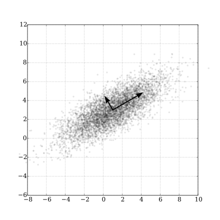
Remarks: In this case, we call $\mathbf{V}$ the loading matrix, and $\mathbf{U}\bs{\Sigma}:=\mathbf{T}$ the score matrix. The PCA scatter plot is thereby the projection onto the PCs, i.e. the columns of $\mathbf{V}$. Specifically, the coordinates are gonna be $\{(t_{ij}, t_{ik})\in\R^2: i=1,2,\ldots, n\}$ namely the selected first columns of the score matrix. This is identical to manually projecting $\mathbf{X}$ onto selected columns of $\mathbf{Q}$ (the principle components) as it can be proved that $t_{ij}=\mathbf{x}_i'\mathbf{q}_j$. However, by using SVD we avoid miss-calculating the eigenvalues in low precision systems.

Definition of Variable PCA

This is merely population PCA on $\mathbf{X}'\in\R^{p\times n}$. Transposing $\mathbf{X}$ swaps the roles of the number of variables and the size of population. The SVD now becomes

$$ \mathbf{X}’ = \mathbf{V}\bs{\Sigma}\mathbf{U}' $$

where we now instead call $\bs{V\Sigma}$ the $\mathbf{T}$ variable.

Remarks: By plotting $\mathbf{X}$ against $\mathbf{V}$ we get PCA scatter plot; by plotting $\mathbf{X}$ against $\mathbf{U}$ on the same piece of paper where draw this PCA scatter plot, we get the so-called biplot.

Application of PCA: Sample Factor Analysis (FA)

One sentence to summarize it: sample factor analysis equals PCA. In formula, FA is trying to write $\mathbf{X}\in\R^p$ into

$$ \mathbf{X} = \bs{\mu} + \mathbf{LF} + \bs{\varepsilon} $$

where $\bs{\mu}\in\R^p$ are $p$ means of features (aka. alphas), $\mathbf{L}\in\R^{p\times m}$ are loadings (aka. betas) and $\mathbf{F}\in\R^m$ are called the factors.

There are some assumptions:

• $m\ll p$ (describing a lot of features in few factors).
• $\E[\mathbf{F}] = 0$ (means are captured already by $\bs{\mu}$), $\Cov[\mathbf{F}]=\mathbf{I}$ (factors are uncorrelated).
• $\E[\bs{\varepsilon}]=0$ (residuals are zero-meaned), $\Cov[\bs{\varepsilon}]=\bs{\Xi}$ is diagonal (residuals are uncorrelated).
• $\Cov[\bs{\varepsilon},\mathbf{F}]=\E[\bs{\varepsilon F}']=\mathbf{O}$ ($ \bs{\varepsilon}$ is uncorrelated with $\mathbf{F}$).

With these assumptions we have $\bs{\Sigma}=\mathbf{LL}'+\bs{\Xi}$.

Canonical Correlation Analysis (CCA)

Similar to PCA, we try to introduce CCA in two ways, namely w.r.t. a population and a sample.

Notations for Population CCA

Assume $p\le q$ (important!!!). Given $\mathbf{X}\in\R^p$ and $\mathbf{Y}\in\R^q$, define

and

Furthermore, define

and

Also, let

Then with this notation we know given $\mathbf{a}\in\R^p$ and $\mathbf{b}\in\R^q$, how expectation, variance and covariance (ans thus correlation) are represented for $U=\mathbf{a}'\mathbf{X}$ and $V=\mathbf{b}'\mathbf{Y}$.

Definition of Population CCA

We calculate canonical correlation variables iteratively:

• $(U_1,V_1)=\arg\max\{\Cov[U,V]:\Var[U]=\Var[V]=1\}$.
• $(U_2,V_2)=\arg\max\{\Cov[U,V]:\Var[U]=\Var[V]=1,\Cov[U,U_1]=\Cov[V,V_1]=\Cov[V,U_1]=\Cov[U,V_1]=0\}$.
• …
• $(U_k,V_k)=\arg\max\{\Cov[U,V]:\Var[U]=\Var[V]=1,\Cov[U,U_i]=\Cov[V,V_i]=\Cov[V,U_i]=\Cov[U,V_i]=0\ \ \forall i=1,2,\ldots, k-1\}$.

Theorem Suppose $p\le q$, let $\Gamma_{\mathbf{XY}}=\bs{\Sigma}_{\mathbf{X}}^{-1/2}\bs{\Sigma}_{\mathbf{XY}}\bs{\Sigma}_{\mathbf{Y}}^{-1/2}\in\R^{p\times q}$ and the condensed SVD be¹

$$ \bs{\Gamma}_{\mathbf{XY}} = \begin{bmatrix} \mathbf{u}_1 & \mathbf{u}_2, & \ldots & \mathbf{u}_p \end{bmatrix}\begin{bmatrix} \sigma_1 & \cdots & \cdots & \mathbf{O} \ \vdots & \sigma_2 & \cdots & \vdots \ \vdots & \vdots & \ddots & \vdots \ \mathbf{O} & \cdots & \cdots & \sigma_p \end{bmatrix}\begin{bmatrix} \mathbf{v}_1’\ \mathbf{v}_2’ \ \vdots \ \mathbf{v}_p' \end{bmatrix} $$

which gives

and that $\rho_k=\sigma_k$.

We call $\rho_k=\Corr[U_k,V_k]$ as the $k$-th population canonical correlation. We call $\mathbf{a}_k=\bs{\Sigma}_{\mathbf{X}}^{-1/2}\mathbf{u}_k$ and $\mathbf{b}_k=\bs{\Sigma}_{\mathbf{Y}}^{-1/2}\mathbf{v}_k$ as the population canonical vectors.

Properties of Population CCA

The canonical correlation variables have the following three basic properties:

• $\Cov[U_i,U_j]=\1{i=j}$.
• $\Cov[V_i,V_j]=\1{i=j}$.
• $\Cov[U_i,V_j]=\1{i=j} \sigma_i$.

Theorem Let $\tilde{\mathbf{X}}=\mathbf{MX}+\mathbf{c}$ be the affine transformation of $\mathbf{X}$. Similarly let $\tilde{\mathbf{Y}}=\mathbf{NY}+\mathbf{d}$. Then by using CCA, the results from analyzing $(\tilde{\mathbf{X}},\tilde{\mathbf{Y}})$ remains unchanged as $(\mathbf{X},\mathbf{Y})$, namely CCA is affine invariant.

Based on this theorem we have the following properties:

• The canonical correlations between $\tilde{\mathbf{X}}$ and $\tilde{\mathbf{Y}}$ are identical to those between $\mathbf{X}$ and $\mathbf{Y}$.
• The canonical correlation vectors are not the same. They now becomes $\tilde{\mathbf{a}_k}=(\mathbf{M}')^{-1}\mathbf{a}_k$ and $\tilde{\mathbf{b}_k}=(\mathbf{N}')^{-1}\mathbf{b}_k$.
• By using covariances $\bs{\Sigma}$ or correlations $\mathbf{P}$ makes no difference in CCA². This is not true for PCA, i.e. there is no simple relationship between PCA obtained from covariances and PCA from correlations.

Example of Calculating Population CCA

Let’s assume $p=q=2$, let

with $|\alpha| < 1$, $|\gamma| < 1$. In order to find the 1st canonical correction of $\mathbf{X}$ and $\mathbf{Y}$, we first check

Therefore, we may calculate

It’s easy to show that $\lambda_1= 2$ and $\lambda_2=0$ are the two eigenvalues of $\bs{11}'$ and thus the 1st canonical correction is

$$ \rho_1 = \sqrt{\frac{4\beta^2}{(1+\alpha)(1+\gamma)}} = \frac{2\beta}{\sqrt{(1+\alpha)(1+\gamma)}}. $$

Notations for Sample CCA

Given $n$ samples: $\mathbf{X}=\{\mathbf{X}(\omega_1), \mathbf{X}(\omega_2), \ldots, \mathbf{X}(\omega_n)\}\in\R^{n\times p}$ and similarly $\mathbf{Y}\in\R^{n\times q}$. Everything is just the same except being in sample notations, e.g. $\bar{\mathbf{X}}=\mathbf{X}'\bs{1} / n$ and $S_{\mathbf{X}}=(\mathbf{X}-\bar{\mathbf{X}}'\bs{1})'(\mathbf{X}-\bar{\mathbf{X}}'\bs{1}) / (n-1)$.

Besides the regular notations, here we also define $r_{\mathbf{XY}}(\mathbf{a},\mathbf{b})$ as the sample correlation of $\mathbf{a}'\mathbf{X}$ and $\mathbf{b}'\mathbf{Y}$:

Definition of Sample CCA

Same as population CCA, we give sample CCA iteratively (except that here we’re talking about canonical correlation vectors directly):

• $(\hat{\mathbf{a}}_1,\hat{\mathbf{b}}_1)=\arg\max\{\mathbf{a}'\mathbf{S}_{\mathbf{XY}}\mathbf{b}:\mathbf{a}'\mathbf{S}_{\mathbf{X}}\mathbf{a}=\mathbf{b}'\mathbf{S}_{\mathbf{Y}}\mathbf{b}=1\}$.
• $(\hat{\mathbf{a}}_2,\hat{\mathbf{b}}_2)=\arg\max\{\mathbf{a}'\mathbf{S}_{\mathbf{XY}}\mathbf{b}:\mathbf{a}'\mathbf{S}_{\mathbf{X}}\mathbf{a}=\mathbf{b}'\mathbf{S}_{\mathbf{Y}}\mathbf{b}=1,\mathbf{a}'\mathbf{S}_{X}\hat{\mathbf{a}}_1=\mathbf{b}'\mathbf{S}_{\mathbf{Y}}\hat{\mathbf{b}}_1=\mathbf{a}'\mathbf{S}_{\mathbf{XY}}\hat{\mathbf{b}}_1=\mathbf{b}'\mathbf{S}_{\mathbf{YX}}\hat{\mathbf{a}}_1=0\}$.
• …
• $(\hat{\mathbf{a}}_k,\hat{\mathbf{b}}_k)=\arg\max\{\mathbf{a}'\mathbf{S}_{\mathbf{XY}}\mathbf{b}:\mathbf{a}'\mathbf{S}_{\mathbf{X}}\mathbf{a}=\mathbf{b}'\mathbf{S}_{\mathbf{Y}}\mathbf{b}=1,\mathbf{a}'\mathbf{S}_{X}\hat{\mathbf{a}}_i=\mathbf{b}'\mathbf{S}_{\mathbf{Y}}\hat{\mathbf{b}}_i=\mathbf{a}'\mathbf{S}_{\mathbf{XY}}\hat{\mathbf{b}}_i=\mathbf{b}'\mathbf{S}_{\mathbf{YX}}\hat{\mathbf{a}}_i=0\}\ \ \forall i=1,2,\ldots,k-1$.

Theorem Given $p\le q$, let $\mathbf{G}_{\mathbf{XY}} = \mathbf{S}_{\mathbf{X}}^{-1/2}\mathbf{S}_{\mathbf{XY}}\mathbf{S}_{\mathbf{Y}}^{-1/2}\in\R^{p\times q}$ and the SVD be

Then we have

In addition,

$$ r_k = r_{\mathbf{XY}}(\hat{\mathbf{a}}_k, \hat{\mathbf{b}}_k) = \sigma_k. $$

We call $r_k$ the $k$-th sample canonical correlation. Also, $\mathbf{Xa}_k$ and $\mathbf{Yb}_k$ are called the score vectors.

Properties of Sample CCA

Everything with population CCA, including the affine invariance, holds with sample CCA, too.

Example of Calculating Sample CCA

Let $p=q=2$, let

$$ \mathbf{X}=\begin{bmatrix} \text{head length of son1}\ \text{head breath of son1} \end{bmatrix}=\begin{bmatrix} l_1\ b_1 \end{bmatrix}\quad\text{and}\quad \mathbf{Y}=\begin{bmatrix} \text{head length of son2}\ \text{head breath of son2} \end{bmatrix}=\begin{bmatrix} l_2\ b_2 \end{bmatrix}. $$

Assume there’re $25$ families, each having $2$ sons. The $\mathbf{W}$ matrix is therefore

$$ \mathbf{W} = \begin{bmatrix} \mathbf{l}_1 & \mathbf{b}_1 & \mathbf{l}_2 & \mathbf{b}_2 \end{bmatrix}\in\R^{25\times 4}. $$

In addition, we may also calculate the correlations $\mathbf{R}_{\mathbf{X}}$, $\mathbf{R}_{\mathbf{Y}}$ and $\mathbf{R}_{\mathbf{XY}}$, from which we have $\mathbf{G}_{\mathbf{XY}}$ given by

which gives the sample canonical correlations $r_1$ and $r_2$ (in most cases $r_1\ll r_2$). In the meantime, we have $\mathbf{u}_{1,2}$ and $\mathbf{v}_{1,2}$ and because of significant difference in scale of $r_1$ and $r_2$, we don’t care about $\mathbf{u}_2$ and $\mathbf{v}_2$. From $\mathbf{u}_1$ and $\mathbf{v}_1$ we can calculate $\hat{\mathbf{a}}_1$ and $\hat{\mathbf{b}}_2$, which indicate the linear relationship between the features. Specifically, the high correlation $r_1$ tells that $\hat{U}_1=\hat{\mathbf{a}}_1\mathbf{X}$ and $\hat{V}_1=\hat{\mathbf{b}}_1\mathbf{Y}$, which are essentially the “girths” (height $+$ breath) of sons’ faces, are highly correlated. In comparison, data shows that $\hat{U}_2$ and $\hat{V}_2$, which describes the “shapes” (height $-$ breath) of sons’ faces, are poorly correlated.

Linear Discriminant Analysis (LDA)

Different from the unsupervised learning algorithms we’ve been discussing in the previous sections, like PCA, FA and CCA, LDA is a supervised classification method in that the number of classes to be divided into is specified explicitly.

Notations for LDA

Assume $g$ different classes $C_1,C_2,\ldots,C_g$. We try to solve the problem asking for the optimal division of $n$ rows of $\mathbf{X}\in\R^{n\times p}$ into $g$ parts: for each $i=1,2,\ldots,g$ denote

with $\sum_{i=1}^g n_i=g$, then given $\mathbf{a}\in\R^p$ we can define

$$ \mathbf{X}_i\mathbf{a} =: \mathbf{y}_i \in \R^{n_i},\quad i=1,2,\ldots,g. $$

Now, recall the mean-centering matrix

$$ \mathbf{H} = \mathbf{I} - \frac{\bs{\iota}\bs{\iota}’}{\bs{\iota}’\bs{\iota}} $$

which provides handy feature that centers a vector by its mean: for any $\mathbf{X}$

$$ \mathbf{HX} = \mathbf{X} - \bs{\iota}’\bar{\mathbf{X}}. $$

With $\mathbf{H}$ we also have the total sum-of-squares as

$$ \mathbf{T} = \mathbf{X}’\mathbf{HX} = \mathbf{X}’\left(\mathbf{I}-\frac{\bs{\iota}\bs{\iota}’}{\bs{\iota}’\bs{\iota}}\right)\mathbf{X} = (n-1)\mathbf{S}. $$

Similarly we define $\mathbf{H}_i$ and $\mathbf{W}_i=\mathbf{X}_i'\mathbf{H}_i\mathbf{X}_i$ for each $i=1,2,\ldots,g$ and thus

where $\mathbf{W}\in\R^{p\times p}$ is known as the within-group sum-of-squares. Finally, check

where we define $\mathbf{B}\in\R^{p\times p}$ as the between-group sum-of-squares.

Theorem For any $\mathbf{a}\in\R^p$, $\mathbf{a}'\mathbf{T}\mathbf{a} = \mathbf{a}'\mathbf{B}\mathbf{a} + \mathbf{a}'\mathbf{W}\mathbf{a}$. However, $\mathbf{T}\neq \mathbf{B}+\mathbf{W}$.

Definition of LDA

First let’s give the Fisher Linear Discriminant Function

$$ f(\mathbf{a}) = \frac{\mathbf{a}’\mathbf{B}\mathbf{a}}{\mathbf{a}’\mathbf{W}\mathbf{a}} $$

by maximizing which, Fisher states, gives the optimal classification.

Theorem Suppose $\mathbf{W}\in\R^{p\times p}$ is nonsingular, let $\mathbf{q}_1\in\R^p$ be the principle eigenvector of $\mathbf{W}^{-1}\mathbf{B}$ corresponding to $\lambda_1=\lambda_{\max}(\mathbf{W}^{-1}\mathbf{B})$, then it can be shown that $\mathbf{q}_1=\arg\max_{\mathbf{a}}f(\mathbf{a})$ and $\lambda_1=\max_{\mathbf{a}}f(\mathbf{a})$.

Proof. We know

$$ \max_{\mathbf{a}} \frac{\mathbf{a}’\mathbf{B}\mathbf{a}}{\mathbf{a}’\mathbf{W}\mathbf{a}} = \max_{\mathbf{a}’\mathbf{W}\mathbf{a}=1} \mathbf{a}’\mathbf{B}\mathbf{a} = \max_{\mathbf{b}’\mathbf{b}=1} \mathbf{b}’\mathbf{W}^{-1/2}\mathbf{B}\mathbf{W}^{-1/2}\mathbf{b} = \lambda_{\max}(\mathbf{W}^{-1/2}\mathbf{B}\mathbf{W}^{-1/2}) = \lambda_{\max}(\mathbf{W}^{-1}\mathbf{B}). $$

Therefore, we have the maximum $\lambda_1$ and thereby we find the maxima $\mathbf{q}_1$.Q.E.D.

Remark: $\lambda_1$ and $\mathbf{q}_1$ can also be seen as the solutions to

$$ \mathbf{B}\mathbf{x} = \lambda \mathbf{W}\mathbf{x},\quad \mathbf{x}\neq\bs{0} $$

which is known as a generalized eigenvalue problem since it reduces to the usual case when $\mathbf{W}=\mathbf{I}$.

Classification Rule of LDA

Given a new data point $\mathbf{t}\in\R^p$ we find

$$ i = \underset{j=1,2,\ldots,g}{\arg\min} |\mathbf{q}_1’(\mathbf{t}-\bar{\mathbf{X}_j})| $$

and assign $\mathbf{t}$ to class $C_j$. This essentially the heuristic behind Fisher’s LDA.

There is no general formulae for $g$-class LDA, but we do have one for specifically $g=2$.

Population LDA for Binary Classification

The population linear discriminant function is

$$ f(\mathbf{a}) = \frac{\sigma_{\text{between}}}{\sigma_{\text{within}}} = \frac{(\mathbf{a}’\bs{\mu}_1 - \mathbf{a}’\bs{\mu}-2)^2}{\mathbf{a}’\bs{\Sigma}_1\mathbf{a} + \mathbf{a}’\bs{\Sigma}_2\mathbf{a}} = \frac{[\mathbf{a}’(\bs{\mu}_1-\bs{\mu}_2)]^2}{\mathbf{a}’(\bs{\Sigma}_1+\bs{\Sigma}_2)\mathbf{a}} $$

which solves to

$$ \mathbf{q}_1 = (\bs{\Sigma}_1 + \bs{\Sigma}_2)^{-1}(\bs{\mu}_1-\bs{\mu}_2) := \bs{\Sigma}^{-1}(\bs{\mu}_1-\bs{\mu}_2) $$

and the threshold

$$ c=\frac{1}{2}(\bs{\mu}_1’\bs{\Sigma}^{-1}\bs{\mu}_1 - \bs{\mu}_2’\bs{\Sigma}^{-1}\bs{\mu}_2). $$

The classification is therefore given by

$$ C(\mathbf{t}) = \begin{cases} C_1\ & \text{if}\quad\mathbf{q}_1’\mathbf{t} > c,\ C_2\ & \text{if}\quad\mathbf{q}_1’\mathbf{t} < c.\ \end{cases} $$

MDS and CA

Variable matrix decomposition methods provide different classes of data analysis tools:

• Based on SVD we have PCA, FA, HITS and LSI for general $\mathbf{A}\in\R^{n\times p}$.
• Based on EVD we have CCA and MDS for $\mathbf{A}\in\R^{p\times p}$, symmetric.
• Based on generalized EVD (GEVD) we have LDA for $\mathbf{A},\mathbf{B}\in\R^{p\times p}$, both symmetric.
• Finally, based on generalized SVD (GSVD) we have CA for $\mathbf{A}=\mathbf{U}\bs{\Sigma}\mathbf{V}'\in\R^{n\times p}$ where we instead of orthonormality of $\mathbf{U}$ and $\mathbf{V}$ assume $\mathbf{U}'\mathbf{D}_1\mathbf{U}=\mathbf{I}$ and $\mathbf{V}'\mathbf{D}_2\mathbf{V}=\mathbf{I}$ for diagonal $\mathbf{D}_1\in\R^{n\times n}$ and $\mathbf{D}_2\in\R^{p\times p}$.