Following are my lecture notes from Prof. Yuri Balasanov’s course Mathematical Market Microstructure.$\newcommand{F}{\mathcal{F}}\newcommand{1}[1]{\unicode{x1D7D9}_{\{#1\}}}\newcommand{Cov}{\text{Cov}}\newcommand{P}{\text{P}}\newcommand{E}{\text{E}}\newcommand{V}{\text{V}}\newcommand{bs}{\boldsymbol}\newcommand{R}{\mathbb{R}}\newcommand{rank}{\text{rank}}\newcommand{\norm}[1]{\left\lVert#1\right\rVert}\newcommand{diag}{\text{diag}}\newcommand{tr}{\text{tr}}\newcommand{braket}[1]{\left\langle#1\right\rangle}\newcommand{C}{\mathbb{C}}\newcommand{d}{\text{d}}$

Introduction

In this section we start with an overview of market microstructure as a whole.

Definition of Market Microstructure

Maureen O’Hara defines market microstructure as

… the study of the process and outcomes of exchanging assets under explicit trading rules. While much of economics abstracts from the mechanics of trading, microstructure literature analyzes how specific trading mechanisms affect the price formation process.

which is generally shown by high frequency trading.

Frog’s Eye View

• (Fundamental Assumption) Central Limit Theorem does not work. Price is not observable unless there’s a trade and thus neither number or size of price movements during a period of time is not garanteed. In fact, no matter how many points we sample from historical data, the mass distribution of price jumps has fatter tails than normal distribution, which means CLT is not working.¹
• (Price Formation and Discovery) Last price is not necessarily an indicator of where it has now formed. Also, price discovery is a destructive experiment involving unique counterpart.
• (Uncertainty Principle) Like quantum mechanics, we can never measure simultaneously price and its volatility manifested in a derivative product. Instead of a number, price is considered a distribution.²
• (The Two Slits Experiment) An order which passed through the previous slit may pass again or be submitted one of the following: hit, lift or join. This activity affacts the state of the trader’ss decision at subsequent times.
• (Technology) Colocated servers; GPS antennas for timing; fiber optics vs. microwave³; Field-Programmable Gate Array (FPGA) and Graphics Processing Unit (GPU); big data.
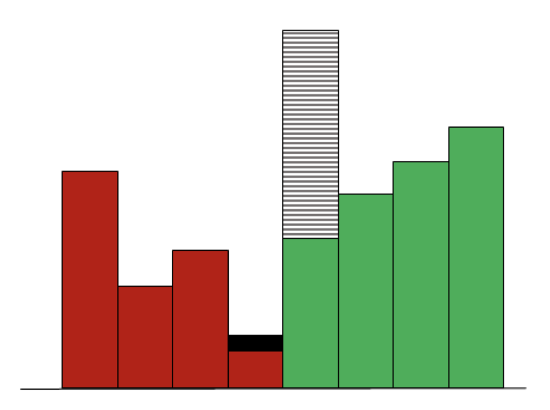
• (Regulation) Spoofing (also see figure below); Rule 610 (locking the market); Dodd-Frank Act⁴ (violation of bids and offers).
• (Future) Direct Market Access (DMA); dark pools; cost of connectivity; speed of light.

Principle of Ma

Ma (間) means empty, spatial void, and interval of space or time in Japanese. The Zen Principle of Ma, when in microstructure context, basically emphasizes that the more “micro” we go into the data, the more randomness we’ll observe.

Characteristics of Transactions Data

• Randomly spaced time intervals (Principle of Ma). Trading intensity contains important information.
• Discrete-valued prices can only be multiples of tick size.
• Diurnal patterns: periodic intensity. For example, high at the beginning and at the end of the trading session.
• To observe microstructure time resolution currently needs to be in microseconds.

Characteristics of Nonsynchronous Trading Data

• Cross-correlation between stock returns at lag 1
• Autocorrelation at lag 1 in portfolio returns
• (Bid-Ask Bounce) Negative autocorrelations in returns of a single stock

Example Stocks A and B are independent. Stock A is traded more frequently than B. News arriving at the very end of day session will more likely a§ect stock A than B. Stock B will react more the next day. Then in daily prices there will be a 1-day lag due to di§erence in trading frequency even when the two stocks are independent.

Models

In this section, we will introduce a series of mathematical models that explain the abovementioned nonsynchronous characteristics.

A Simple Model to Start With

Let $r_t$ be continuously compounded return at time $t$. Assume that $r_t$ are i.i.d. latent variables, $\E[r_t] = μ$, $\V[r_t]=\sigma$. For each $t$ probability that the asset is not traded is $\pi$. Let $r_t^0$ be the manifest return variable. If at $t$ there is no trade $r_t^0 = 0$. If at $t$ there is a trade then $r_t^0$ is the cumulative return since the previous trade.

It can be shown that

This simple model explains negative autocorrelation induced by nonsynchronous trading.

Ordered Probit Model

Let $y_t$ be a latent variable depending on time. Observed variable is $u_t$. Assume $u_t$ is an ordered $k$-categorical variable:

$$ u_t = \begin{cases} u^{(0)} & \text{if }y_t\in (-\infty,\theta_1),\ u^{(i)} & \text{if }y_t\in [\theta_i,\theta_{i+1}),\ i=1,2,\ldots,k-1,\ u^{(k)} & \text{if }y_t\in [\theta_k,\infty). \end{cases} $$

Variable $y_t$ is predicted using a linear model $y_t=\bs{\beta}\mathbf{X}_t + \epsilon_t$, which gives

Note here we assume $\epsilon_t\sim\mathcal{N}(0,\sigma_t^2)$ and thus applied $\Phi(\cdot)$ as link function, which explains why it’s a Probit model.

Decomposition Model

Assume the price change $y_i = P_{t_i} - P_{t_{i-1}}$ can be decomposed into product of three components:

• Indicator of price change $A_i\in\{0,1\}$.
• Direction of price change $D_i\in\{-1,+1\}$.
• Size of price change $S_i\in\mathbb{N}_+$.

Specifically, for $p_i=\P[A_i=1]$ we let

For $\delta_i=\P[D_i=1\mid A_i=1]$ we let

For $S_i$ we let

where $g(\lambda_{\xi,i})$ is geometric distribution with parameter $\lambda_{\xi,i}$ estimated from

Examples We can choose features as below

from which we can train a simple decomposition model using in-sample data.

Hawkes Model

We can model the price as a compound Cox process and use Hawkes model to estimate it. For definition and detailed analysis check out the next section.

Stochastic Processes

Let’s first define two basic processes: Markov process and point process.

Markov Process

$Y$ is called a Markov process if

$$ \P[Y_t\le y\mid \F_s^Y] = \P[Y_t\le y\mid Y_s] $$

$\P$-a.s. for all $t\ge s\ge 0$ and $y\in\R$.

Point Process

Let $\mathcal{N}$ be a set of all right-continuous non-decreasing integer-valued functions $\{v(t):v_0= 0; t\ge 0\}$. Any random variable $N(t)$ with trajectories from $\mathcal{N}$ is called a point process. It can also be seen as the counting process of random events.

Property (Stationarity) A point process is stationary if $\Delta_s=N(s+t)-N(s)$ has the same distribution for all $s$.

Poisson Process

Before defining the Poisson process, let’s review some basics about Poisson distribution.

(Poisson Distribution) We say $N\sim\text{Pois}(\lambda)$ if

$$ \pi_{\lambda,k} \equiv \P[N=k] = \frac{\lambda^k e^{-\lambda}}{k!} $$

where it can be proved that $\E[N]=\V[N]=\lambda$. Poisson distribution is in fact a small probability limit of binomial distribution.

(Mixed Poisson Distribution) Let’s say $N\sim \text{Pois}(\lambda t)$ and $\Lambda$ be a random variable with distribution $\text{U}$. Now instead of sticking with constant $\lambda$, assume random $\Lambda$ as intensity and we have mixed Poisson distribution

$$ p_k(t) \equiv \P[N=k] = \E!\left[\frac{(\Lambda t)^k e^{-\Lambda t}}{k!}\right] = \int_0^{\infty} \frac{(\lambda t)^k e^{-\lambda t}}{k!}\d \text{U} = \int_0^{\infty} \frac{(\lambda t)^k e^{-\lambda t}}{k!}u(\lambda)\d\lambda. $$

Extend this to the joint distribution of $(N,\Lambda)$ and we have

$$ \P[N=k,\Lambda\le x] = \int_0^x \frac{(\lambda t)^k e^{-\lambda t}}{k!} \d\text{U},\quad x \ge 0. $$

Assume

$$ \E[\Lambda] = \mu_{\Lambda},\quad \V[\Lambda] = \sigma_{\Lambda}^2 $$

then

$$ \E[N] = t\mu_{\Lambda},\quad \V[N] = t\mu_{\Lambda} + t^2\sigma_{\Lambda}^2 \ge t\mu_{\Lambda}. $$

This is called over-dispersion (variance greater than expectation).

Example If we use Gamma distribution as the structure distribution for a mixed Poisson distribution, then

$$ u(\lambda) = \frac{\beta^{\alpha}}{\Gamma(\alpha)}\lambda^{\alpha-1} e^{-\beta \lambda} $$

where $\lambda \ge 0$, $\alpha,\beta>0$ and

$$ \Gamma(\alpha) = \int_0^{\infty} x^{\alpha - 1}e^{-x}\d x,\quad \alpha > 0 $$

with $\alpha$ being called the shape parameter and $\beta$ called the scale parameter. When $\beta=1$ it’s a standard Gamma distribution; when $\alpha=1$ it’s an exponential distribution; when $\alpha=k\in\mathbb{N}_+$, the distribution is the sum of $k$ exponential r.v.s.

For $\Lambda\sim\text{Gamma}(\alpha,\beta)$, we have

$$ \E[\Lambda] = \mu_{\Lambda} = \frac{\alpha}{\beta},\quad\V[\Lambda] = \sigma_{\Lambda} = \frac{\alpha}{\beta^2} $$

and for the corresponding mixed distribution

$$ \begin{align} \P[N=k] &= \binom{\alpha+k-1}{k}\left(\frac{\beta}{\beta + k}\right)^{\alpha}\left(\frac{t}{\beta+t}\right)^k\ &\overset{\alpha=1}{=} \frac{\beta}{\beta+t}\left(\frac{t}{\beta+t}\right)^k \end{align}. $$

Definition (Poisson Process) A point process $N(t)$ is called a Poisson process with intensity $\lambda$ if:

• $N(t)$ has independent increments.
• $N(t)-N(s)\sim\text{Pois}(\lambda(t-s))$ for any $t\ge s\ge 0$.

Definition (Non-Homogeneous Poisson Process) A point process $N_A(t)$ is called a non-homogeneous Poisson process with intensity measure $A_t\in\mathcal{A}$ if

• $N_A(t)$ has independent increments.
• $N_A(t) - N_A(s)\sim\text{Pois}(A_t-A_s)$.

Cox Process

Let $\Lambda_t$, $t\ge 0$, be a random process with trajectories from $\mathcal{A}$. Cox process is a generalization of non-homogeneous Poisson process in which intensity measure can be stochastic in a certain way.

Definition (Cox Process) A point process $N_{\Lambda}(t)$ is called Cox process with random intensity measure $\Lambda_t$ if for any realization $A_t$ of $\Lambda_t$ the process $N_{\Lambda}(t)$ is a non-homogeneous Poisson process with intensity measure $A_t$.

Definition of Cox process means that we can generate Cox process by first generating a trajectory of intensity measure $A_t$ and then generating trajectory of $N_{\Lambda}(t)$ as a trajectory of non-homogeneous Poisson process with intensity measure $A_t$. If $N_1(t)$ is a homogeneous Poisson process with unit intensity independent of random intensity measure $\Lambda_t$ then Cox process $N_{\Lambda}(t)$ is a superposition of $N_1(t)$ and $\Lambda_t$:

$$ N_{\Lambda}(t) = N_1(\Lambda_t),\quad t\ge 0. $$

Definition (Compound Cox Process) Let $X_1,X_2,\ldots$ be i.i.d. and have at least two moments, say $\E[X]=a$, $\V[X]=\sigma^2<\infty$. Let $N(t)=N(\Lambda_t)$ be a Cox process independent of $X$, then

$$ S(t) := \sum_{i=1}^{N(\Lambda_t)} X_i,\quad t \ge 0 $$

is called a compound Cox process. It can be derived $\E[S]=a\mu_{\Lambda}$, $\V[S]=(a^2+\sigma^2)\mu_{\Lambda} + a^2\sigma_{\Lambda}^2$.

Particularly, when $\Lambda_t = \lambda t$, $S(t)$ is a compound Poisson process.

Theorem (Central Limit Theorem for Compound Cox Processes) Let $\Lambda_t\overset{p}{\to} \infty$, for weak convergence to some random variable $Z$ given by

$$ \frac{S(t)}{\sigma_X\sqrt{d(t)}}\to Z,\quad t\to \infty $$

where $d(t)$ is a strictly increasing function on time $t$ and $d(t)\equiv t$ when we assume calendar time i.e. time flowing minute by minute, it’s necessary and sufficient that

• $\P[Z< z] = \int_0^{\infty}\Phi(zy^{-\frac{1}{2}})\d \P[U< u]=\E[\Phi(zU^{-\frac{1}{2}})]$, $z\in\R$.
• $\frac{\Lambda_t}{d(t)}\to U$, $t\to \infty$.

Note that the asymptotic distribution $\Lambda_t / \d t$ does not depend on $t$ but can still be stochastic. The limit distribution is not Gamma, but rather a mixed one that can be very heavy tailed in many cases, which explains why CLT doesn’t work in finance. In fact, CLT holds if and only if the limit distribution $U$ is constant $1$.

Example (Dynamic VaR) Assuming that cumulative intensity process $\Lambda(t)$ is a Gamma process (i.e. a process starting from $0$ with independent increments distributed as Gamma distribution) the $q$-level quantile of the maximum loss distribution is calculated as

$$ D(T,q) = \sigma\sqrt{\frac{\mu T}{2}}\ln\left(\frac{1}{1-q}\right). $$

Hawkes Process

A Hawkes process $N_t$, also known as a self-exciting counting process, is a simple point process whose conditional intensity can be expressed as

$$ \begin{align} \lambda(t) &= \mu (t) + \int_{- \infty}^t \nu (t - s) d N_s\ &= \mu (t) + \sum_{T_k < t} \nu (t - T_k) \end{align} $$

where $\nu : \mathbb{R}^+ \rightarrow \mathbb{R}^+$ is a kernel function which expresses the positive influence of past events $T_i$ on the current value of the intensity process $\lambda (t)$, $\mu (t)$ is a possibly non-stationary function representing the expected, predictable, or deterministic part of the intensity, and $\{ T_i : T_i < T_{i + 1} \} \in \mathbb{R}$ is the time of occurrence of the i-th event of the process.

Specifically, when we use exponential decay with parameter (which is also the most famous type of Hawkes processes), the formulation becomes

$$ \Lambda_t = \lambda + \sum_{0\le T_k\le t} \alpha \exp[-\beta(t-T_k)],\quad t\ge 0. $$

Branching Process

Consider a random model for population growth in the absence of spatial or any other resource constraints. In such population of individuals in every generation $n=0,1,2,\ldots$, each individual produces a random number $h$ of children in the next generation, independently of other individuals.⁵ The probability distribution function for children in the next generation is often called the offspring distribution and is given by $p_i=\P[h=i]$ for $i=1,2,\ldots$.

There can be two cases:

• (w/o immigration) This Markov chain has only one absorbing state, i.e. $0$ and all other states are transient if $p_0>0$. The population either dies out or goes to infinity.

• (w/ immigration) If we assume immigrants join the population by Pois$(\lambda)$, and say that the offspring distribution for immigrants are Binom$(1,p)$, then the total number of new immigrant children follows Pois$(\frac{\lambda}{1-p})$. In this case, there is possibility of a limiting distribution for the population size.

Hawkes process can be seen as a branching process with immigration. For Hawkes process the branching ratio is defined as the ratio of $\alpha$ the excitability to $\beta$ the decay.