Literature Review on Optimal Order Execution (3)

2018-04-29

Here I’m trying to write something partly based on Cont’s first model in the previous post. I plan to skip the Laplace transform and go for Monte Carlo simulation. Also, I’m trying to abandon the assumption of unified order sizes. To implement that, I need to shift from a Markov chain which is supported by discrete spaces, onto some other stochastic process that is estimatable. Moreover, although I actually considered supervised learning for this problem, I gave it up at last. This is because my model is inherently designed for high frequency trading and thus training for several minutes each time would be intolerable.

Section 1: Package Import

import smm
import numpy as np
import scipy as sp
import pandas as pd
import matplotlib.pyplot as plt
from scipy import special
from scipy.optimize import brute
from scipy.stats import skellam, t, kurtosis, gaussian_kde
from matplotlib.patches import Patch

np.set_printoptions(linewidth=200)
pd.set_option('display.max_rows', 20)
%config InlineBackend.figure_format = 'retina'

I need smm for multivariate stochastic processes, and scipy.optimize for maximum likelihood estimation.

def retrieve_data(date):
    file = 'data/depth_quarter_200_{}.csv'.format(date)
    data = pd.read_csv(file)
    return data


date = '20180129'
data.columns = ['time'] + list(data.columns[1:])
data.head()

	time	ask_price_1	ask_price_10	ask_price_100	ask_price_101	ask_price_102	ask_price_103	ask_price_104	ask_price_105	ask_price_106	…	bid_vol_90	bid_vol_91	bid_vol_92	bid_vol_93	bid_vol_94	bid_vol_95	bid_vol_96	bid_vol_97	bid_vol_98	bid_vol_99
1	2018-01-29 00:00:06.951631+08:00	12688.00	12663.58	12391.48	12390.00	12389.96	12388.00	12384.22	12381.39	12380.00	…	6.0	15.0	1.0	460.0	4.0	121.0	5.0	1.0	5.0	120.0
2	2018-01-29 00:00:07.792882+08:00	12676.93	12657.04	12391.48	12390.00	12389.96	12388.00	12384.22	12381.39	12380.00	…	1.0	400.0	363.0	5.0	6.0	15.0	1.0	460.0	4.0	121.0
3	2018-01-29 00:00:08.702945+08:00	12643.27	12617.26	12361.27	12360.00	12359.38	12358.06	12356.22	12355.44	12354.17	…	6.0	15.0	1.0	460.0	4.0	121.0	5.0	1.0	5.0	120.0
4	2018-01-29 00:00:10.998615+08:00	12666.00	12642.73	12380.00	12377.00	12374.99	12369.73	12366.43	12365.84	12361.45	…	460.0	4.0	121.0	5.0	1.0	5.0	120.0	150.0	12.0	97.0
5	2018-01-29 00:00:11.742304+08:00	12674.00	12643.27	12384.22	12381.39	12380.00	12377.00	12374.99	12369.73	12366.43	…	4.0	121.0	5.0	60.0	1.0	5.0	120.0	150.0	12.0	97.0

Larger index means smaller values for both bid and ask prices. It’s uncommon and here I re-indexed the variables s.t. bid_1 and ask_1 corresponds with the best opponent prices.

def rename_index(s):
    if 'ask' in s:
        _, v, i = s.split('_')
        return f'ask_{v}_{200 - int(i) + 1}'
    else:
        return s

data.columns = list(map(rename_index, data.columns))

Section 2: Data Mining

variables = list(data.columns[1:])

I dropped the time variable simply because I don’t know how to use it. Normally there’re two ways to handle uneven time-grids: resampling and ignoring, and I chose the latter.

def plot_lob(n, t, theme='w'):
    # function to plot the limit order book
    assert theme in ['w', 'k', 'white', 'black']

    temp_price = data[[f'bid_price_{i}' for i in range(n, 0, -1)] + \
                      [f'ask_price_{i}' for i in range(1, n + 1)]].head(t)
    temp_vol = data[[f'bid_vol_{i}' for i in range(n, 0, -1)] + \
                    [f'ask_vol_{i}' for i in range(1, n + 1)]].head(t)
    for i in range(1, n):
        temp_vol.iloc[:, n + i] += temp_vol.iloc[:, n + i - 1]
    for i in range(1, n):
        temp_vol.iloc[:, n - i - 1] += temp_vol.iloc[:, n - i]
    price_min, price_max = temp_price.min().min(), temp_price.max().max()
    price_limits = (price_min * 1.1 - price_max * .1, price_max * 1.1 - price_min * .1)

    fig = plt.figure(figsize=(12, 6))

    fc1 = theme
    ax1 = plt.subplot2grid((5, 1), (0, 0), rowspan=4, facecolor=fc1)
    ax1.fill_betweenx(x1=n - 1, x2=n, y=price_limits, color='r', alpha=.2, lw=0)
    lc = 'k' if theme in ['w', 'white'] else 'w'
    for i in range(t):
        ax1.plot(temp_price.iloc[i, :].values, color=lc, alpha=(i + 1) / t, lw=1)
    ax1.set_ylim(price_limits)
    ax1.set_xticklabels('')
    ax1.spines['bottom'].set_visible(False)
    ax1.set_ylabel('price')
    ax1.set_xlim(-.5, 2 * n - .5)

    fc2 = '#efefef' if theme in ['w', 'white'] else '#222222'
    ax2 = plt.subplot2grid((5, 1), (4, 0), facecolor=fc2)
    ax2.fill_betweenx(x1=n - 1, x2=n, y=[0, temp_vol.max().max() * 1.1], color='r', alpha=.2, lw=0)
    for i in range(t):
        ax2.bar(np.arange(2 * n), temp_vol.iloc[i, :].values, color=lc, alpha=.2)
    ax2.set_ylim(0, temp_vol.max().max() * 1.1)
    ax2.spines['top'].set_visible(False)
    ax2.set_ylabel('volume')
    ax2.set_xlim(-.5, 2 * n - .5)
    ax2.set_xticks(range(2 * n))
    ax2.set_xticklabels([f'bid_{i}' for i in range(n, 0, -1)] + \
                        [f'ask_{i}' for i in range(1, n + 1)], rotation=90)

    plt.tight_layout()
    plt.subplots_adjust(hspace=.0)
    plt.show()

Now we make a plot of the order book within the past 10 steps, including 20 bid levels and 20 ask levels.

n, t = 20, 10
plot_lob(n, t)

png

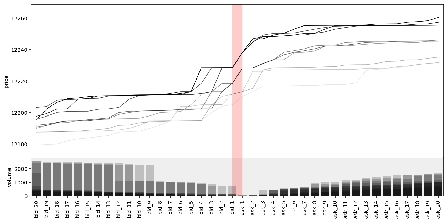
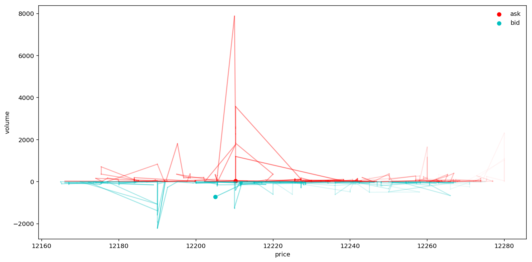
Not sure if it tells any critical information. Let’s make another plot. This time $t=500$ and we only consider the best bid and ask orders.

fig = plt.figure(figsize=(12, 6))
ax = fig.add_subplot(111)
# ax.set_yscale('log')
ax.set_xlabel('price')
ax.set_ylabel('volume')

t = 500

ap = data['ask_price_1'].values
av = data['ask_vol_1'].values
ax.scatter(ap[0], av[0], color='r', label='ask')
for i in range(t):
    ax.plot((ap[i], ap[i + 1]), (av[i], av[i + 1]), 'r-', alpha=(1 - i / t) * .5)

bp = data['bid_price_1'].values
bv = data['bid_vol_1'].values
ax.scatter(bp[0], -bv[0], color='c', label='bid')
for i in range(t):
    ax.plot((bp[i], bp[i + 1]), (-bv[i], -bv[i + 1]), 'c-', alpha=(1 - i / t) * .5)

plt.legend(loc='best', frameon=False)    
plt.tight_layout()
plt.show()

png

price = data[[f'bid_price_{i}' for i in range(n,0,-1)] + [f'ask_price_{i}' for i in range(1,n+1)]]
vol = data[[f'bid_vol_{i}' for i in range(n,0,-1)] + [f'ask_vol_{i}' for i in range(1,n+1)]]

A simple idea would be inputting the prices and volumes in the current orderbook, and predict the future mid prices. Furthermore, it’s ideal to have a rough expectation of the minimum time that the mid price crosses a certain price, or the time needed in expectation before my order got executed successfully.

change = []
for i in range(price.shape[0] - 1):
    # print(f'checking state {i} and {i+1}', end='\r')
    mask = np.isin(price.iloc[i + 1, :].values, price.iloc[i, :].values) + \
           np.isin(price.iloc[i, :].values, price.iloc[i + 1, :].values)
    cnames = price.columns[mask]
    mask = list(map(lambda x: x.replace('price', 'vol'), cnames))
    change1 = vol[mask].iloc[i + 1] - vol[mask].iloc[i]
    cnames = [c for c in price.columns if c not in cnames]
    mask = list(map(lambda x: x.replace('price', 'vol'), cnames))
    change2 = vol[mask].iloc[i + 1] - vol[mask].iloc[i]
    change_temp = np.zeros(2 * n)
    for ci in range(2 * n):
        c = vol.columns[ci]
        if c in change1:
            change_temp[ci] += change1[c]
        if c in change2:
            change_temp[ci] += change2[c]
    change.append(change_temp)

The calculation of change took over 10 minutes. I don’t think it’s gonna be useful in real work. However, it’s not so bad an idea to save it somewhere locally in case I need it later.

change = pd.DataFrame(np.array(change).astype(int), columns=vol.columns)
change.to_csv(f'data/change_{date}.csv')

Section 3: Model

change = pd.read_csv(f'data/change_{date}.csv', index_col=0)

After some research, I decided to fit the data in change to student’s t-distribution, Skellam distribution, and two-side Weibull distribution. I’ll now elaborate reason why I chose, and how to estimate each distribution below.

First is the t-distribution. It is well-known for its leptokurtosis which suits well in many financial time series as a better alternative to Normal distribution. The PDF and CDF of the t-distribution involves the Gamma function and thus would be computationally troublesome when we want to calculate the MSE of the parameters. However, notice for any r.v. $X\sim t(\nu,\mu,\sigma)$ , we have relationship

$$ \text{Var}(X) = \begin{cases} \frac{\nu}{\nu - 2} & \text{for }\nu > 2,\\ \infty & \text{for }1 < \nu \le 2,\\ \text{undefined} & \text{otherwise} \end{cases} $$

and

$$ \text{Kur}_+(X) = \begin{cases} \frac{6}{\nu - 4} & \text{for }\nu > 4,\\ \infty & \text{for }2 < \nu \le 4,\\ \text{undefined} & \text{otherwise} \end{cases} $$

where $\text{Kur}_+\equiv \text{Kur} - 3$ is the excess kurtosis, we can simply go for moment estimation for t-distribution using empirical variance or kurtosis.

Second, the Skellam distribution. This is mainly due to the original model used in Cont’s paper, where he assumes Poisson order arrivals uniformly over the time. Here I slightly improve the model s.t. bid and ask orders are modelled in the same time and represented by r.v. $S\equiv P_a - P_b$ where $P_a\sim Pois(\lambda_a)$ and $P_b\sim Pois(\lambda_b)$ . This is therefore a discrete distribution with two parameters. scipy.stats has its PMF implemented and all I need to do is numerically maximize the likelihood.

For the two-sided Weibull distribution, it is given by

$$ Y = \begin{cases} -\text{Weibull}(\lambda_1, k_1) & \text{if } Y < 0,\\ \text{Weibull}(\lambda_2, k_2) & \text{otherwise} \end{cases} $$

where shape parameters $k_{1,2}\ge 0 $ and scale parameters $\lambda_{1,2} > 0$ .

Therefore, the pdf is

$$ f(y \mid \lambda_1, k_1, \lambda_2, k_2) = \begin{cases} \left(\frac{-y}{(\lambda_1)}\right)^{k_1 -1}\exp\left(-\left(\frac{-y}{(\lambda_1)}\right)^{k_1}\right) & \text{if y < 0},\\ \left(\frac{y}{(\lambda_2}\right)^{k_2 -1}\exp\left(-\left(\frac{y}{(\lambda_2)}\right)^{k_2}\right) & \text{otherwise} \end{cases} $$

and to normalize the integration to $1$ , we also have

$$ \frac{\lambda_1}{k_1} + \frac{\lambda_2}{k_2} = 1 \Rightarrow \lambda_2 = k_2 (1 - \lambda_1 / k_1) $$

which means there’re in fact only three parameters to estimate.

Now we rewrite the log-likelihood as

$$ \begin{align*} LL = \sum_{i=1}^n \log(f(y_i)) = \sum_{i=1}^n &\left((k_1-1)(\log^*(-y_i) - \log^*(\lambda_1)) - (-y_i / \lambda_1)^{k_1}\right)\mathbb{I}_{y_i < 0} + \\ &\left((k_2-1)(\log^*(y_i) - \log^*(\lambda_2)) - (y_i / \lambda_2)^{k_2}\right)\mathbb{I}_{y_i \ge 0}. \end{align*} $$

where we have the special $\log^*(y)\equiv 0$ if $y\le0$ .

i = 15  # take ask_15 for example

fig = plt.figure(figsize=(12, 6))

ax = fig.add_subplot(111)

cgrid = np.array([c for c in change[f'bid_vol_{-i}' if i < 0 \
                  else f'ask_vol_{i}'] if -200 < c < 200])[::200]
cgrid.sort()
density = gaussian_kde(cgrid)
ax.plot(cgrid, density(cgrid), 'r-', label='gaussian')

exkur = kurtosis(cgrid) - 3
scale1 = np.std(cgrid)
scale2 = (2 - 6 / (6 + 2 * exkur))**.5
params = [6 / exkur + 4, np.mean(cgrid), scale1 * .3 + scale2 * .7]
ax.plot(cgrid, t.pdf(cgrid, *params), 'c-', label='t({:.2f}, {:.2f}, {:.2f})'.format(*params))

negloglik_skellam = lambda mu: -sum(skellam.logpmf(cgrid, *mu))
mu = brute(negloglik_skellam, ranges=[(100, 500), (100, 500)], Ns=10, finish=None)
ax.plot(cgrid, skellam.pmf(cgrid, *mu), 'y-', label='skellam({:.2f}, {:.2f})'.format(*mu))

# log_ = lambda y: np.log(y) if y > 0 else 0
# def logpdf_tweibull(y, params):
#     l1, k1, k2 = params
#     l2 = k2 * (1 - l1 / k1)
#     if l1 >= k1 or l2 >= k2:
#         return 1e5
#     ret = float(((k1 - 1) * (log_(-y) - log_(l1)) - (-y / l1)**k1) * (y < 0) + \
#                 ((k2 - 1) * (log_(y) - log_(l2)) - (y / l2)**k2) * (y >= 0))
#     if np.isnan(ret):
#         return 1e5
#     return ret
# negloglik_tweibull = lambda params: -sum(logpdf_tweibull(y, params) for y in cgrid / 1000)
# params = brute(negloglik_tweibull, ranges=[(.1, .9), (.1, .9), (.1, .9)], Ns=10, finish=None)
# l1, k1, k2 = params
# l2 = k2 * (1 - l1 / k1)
# params = np.array([l1, k1, l2, k2]); print(params)
# tweibull_pdf = lambda y: (-y/l1)**(k1-1)*np.exp(-(-y/l1)**k1) * (y < 0) + \
#                          (y/l2)**(k2-1)*np.exp(-(y/l2)**k2) * (y >= 0)
# tweibull_cdf = np.cumsum([tweibull_pdf(y) for y in cgrid / 1000])
# ax.plot(cgrid, tweibull_cdf, 'b-', label='tweibull({:.2f}, {:.2f}, {:.2f}, {:.2f})'.format(*params))

ax.hist(cgrid, bins=40, facecolor=(0,0,0,.5), edgecolor='k', normed=True, label='change')
ax.set_xlim(-200, 200)
ax.set_xlabel('change')

plt.legend(loc='best', frameon=False)
plt.tight_layout()
plt.show()

png

As coded above, at last I didn’t include two-sided Weibull distribution because the optimization did not converge. In conclusion, for changes of order sizes (denoted by $x$ ), we use modified t-distribution with

$$ \hat{\mu} = \bar{x},\quad \hat{\sigma} = 0.3 \cdot \sqrt{\widehat{\text{Var}}(x)} + 0.7 \cdot \sqrt{\left(2 - \frac{6}{6 + 2\ \widehat{\text{Kur}}_+(x)}\right)} $$

and

$$ \hat{\nu} = \frac{6}{\widehat{\text{Kur}}_+(x)} + 4 $$

where

$$ \widehat{\text{Kur}}_+(x) = \widehat{\text{Kur}}(x) - 3 $$

while

$$ \widehat{\text{Kur}}(x) = \hat{m}_4(x) / \hat{m}_2^2(x) $$

and

$$ \hat{m}_4 = \sum_{i=1}^n (x_i - \bar{x})^4 / n,\quad \hat{m}_2 = \sum_{i=1}^n (x_i - \bar{x})^2 / n. $$

Now, when we assume independence across different buckets of order book, we can estimate the parameters of t-distributions as below.

params = np.zeros([2 * n, 3])
nrow = 0
for i in np.arange(-n, n + 1):
    if not i: continue
    cgrid = np.array([c for c in change[f'bid_vol_{-i}' if i < 0 \
                      else f'ask_vol_{i}'] if -200 < c < 200])[::200]
    exkur = kurtosis(cgrid) - 3
    scale1 = np.std(cgrid)
    scale2 = (2 - 6 / (6 + 2 * exkur))**.5
    params[nrow,:] = [6 / exkur + 4, np.mean(cgrid), scale1 * .3 + scale2 * .7]
    nrow += 1

params

array([[ 5.1589201 , -0.52536232, 11.05729   ],
       [ 5.86412495, -0.61454545, 12.08484143],
       [ 5.82376701,  4.61231884, 11.67543236],
       [ 6.28819815, -0.7173913 , 10.85941723],
       [ 6.89178374, -1.59927798, 11.25140225],
       [ 6.14231284,  2.29856115, 12.46686452],
       [ 6.4347771 ,  2.22302158, 13.73785226],
       [ 6.17737187,  0.67753623, 12.19098061],
       [ 5.9250571 , -1.68231047, 12.54472066],
       [ 5.16886809, -0.69090909, 11.94199489],
       ...
       [ 5.94772822,  3.18181818, 12.4415555 ],
       [ 6.5157695 ,  4.62181818, 13.67098387],
       [ 6.69385395,  0.66304348, 13.63770319],
       [ 4.99329442, -1.11510791, 11.63780506],
       [ 5.04144977,  1.91756272, 11.20026029],
       [ 5.47054269, -4.34163701, 10.66971035],
       [ 5.11684414, -2.35460993,  9.98656422],
       [ 4.89130697,  1.07092199, 11.5511127 ],
       [ 5.31202782, -0.58865248, 11.01769165],
       [ 5.17908162,  2.16961131, 10.81368767]])

When we do not ignore the correlation across all buckets, a multivariate t-distribution must be considered. Similar to multivariate Normal distributions, here we need to estimate a covariance matrix, a vector of expectations and a vector of degrees of freedom. Notice the degrees of freedom do not vary significantly across the rows in params, to accelerate computation I set a unified degree of freedom for all buckets, namely $df = 7$ . Using Expectation Maximization (EM) algorithm introduced by D. Peel and G. J. McLachlan (2000), I wrote the model below to estimate this distribution.

class MVT:
    def __init__(self, df=3.5):
        self.df = df

    def fit(self, X, iter=200, eps=1e-6):
        # initialize parameters
        D = X.shape[1]
        N = X.shape[0]
        cov = np.cov(X, rowvar=False)
        mean = X.mean(axis=0)
        mu = X - mean[None, :]
        delta = np.einsum('ij,ij->i', mu, np.linalg.solve(cov, mu.T).T)
        z = (self.df + D) / (self.df + delta)
        obj = [
            -N * np.linalg.slogdet(cov)[1] / 2 - (z * delta).sum() / 2
            -N * special.gammaln(self.df / 2) + N * self.df * np.log(self.df / 2) / 2
            +self.df * (np.log(z) - z).sum() / 2
        ]

        # iterate EM algorithm
        for i in range(iter):
            # M step
            mean = (X * z[:, None]).sum(axis=0).reshape(-1, 1) / z.sum()
            mu = X - mean.squeeze()[None, :]
            cov = np.einsum('ij,ik->jk', mu, mu * z[:, None]) / N

            # E step
            delta = (mu * np.linalg.solve(cov, mu.T).T).sum(axis=1)
            delta = np.einsum('ij,ij->i', mu, np.linalg.solve(cov, mu.T).T)
            z = (self.df + D) / (self.df + delta)

            # store objective
            obj.append(
                -N * np.linalg.slogdet(cov)[1] / 2 - (z * delta).sum() / 2
                -N * special.gammaln(self.df / 2) + N * self.df * np.log(self.df / 2) / 2
                +self.df * (np.log(z) - z).sum() / 2
            )
            err = np.abs(obj[-1] - obj[-2])
            print(f'Iteration {i + 1}')
            if err < eps: break
        return cov, mean.squeeze()


model = MVT(7)
S, m = model.fit(change.values)

Now the distribution for order size movement is estimated. We can simulate the trajectory and rebuild the order book in future several steps. Specifically, notice the predicted movement may well change the shape of the order book while, according to practical observation, the order book retains its “V”-shape in most of the time. Therefore, I sort up separately both halves of the order book every time they’re updated by a predicted order size movement (or “co-movement”, since it should be a vector).

n_steps = 20
prediction = smm.smm.SMM.multivariate_t_rvs(S=S, m=m, df=7, n=n_steps)
orderbook = np.zeros([1 + n_steps, 2 * n])
orderbook[0,:] = 0
for i in range(1, n_steps + 1):
    orderbook[i, :n] = np.sort(orderbook[i - 1, :n] + prediction[i - 1, :n])[::-1]
    orderbook[i, n:] = np.sort(orderbook[i - 1, n:] + prediction[i - 1, n:])

Below is a simple sketch of this order book trajectory where I assign stronger color to the traces that are closer to the best (bid/ask) prices.

fig = plt.figure(figsize=(12, 6))
ax = fig.add_subplot(111)
for i in range(n):  # stronger color means closer to mid price
    ax.plot(range(1 + n_steps), orderbook[:,i], 'r-', alpha=(i + 1) / n)
for i in range(n, 2 * n):  # stronger color means closer to mid price
    ax.plot(range(1 + n_steps), orderbook[:,i], 'c-', alpha=(2 * n - i) / n)
ax.set_xticks(range(n_steps + 1))
ax.set_xlabel('evolution')
ax.set_ylabel('order book')
plt.tight_layout();

png

It can be seen from the figure that stronger traces are located more to the bottom, which validates our intuition since trades around the current price are more active than those to the left or the right of the order book.

Section 4: Prediction

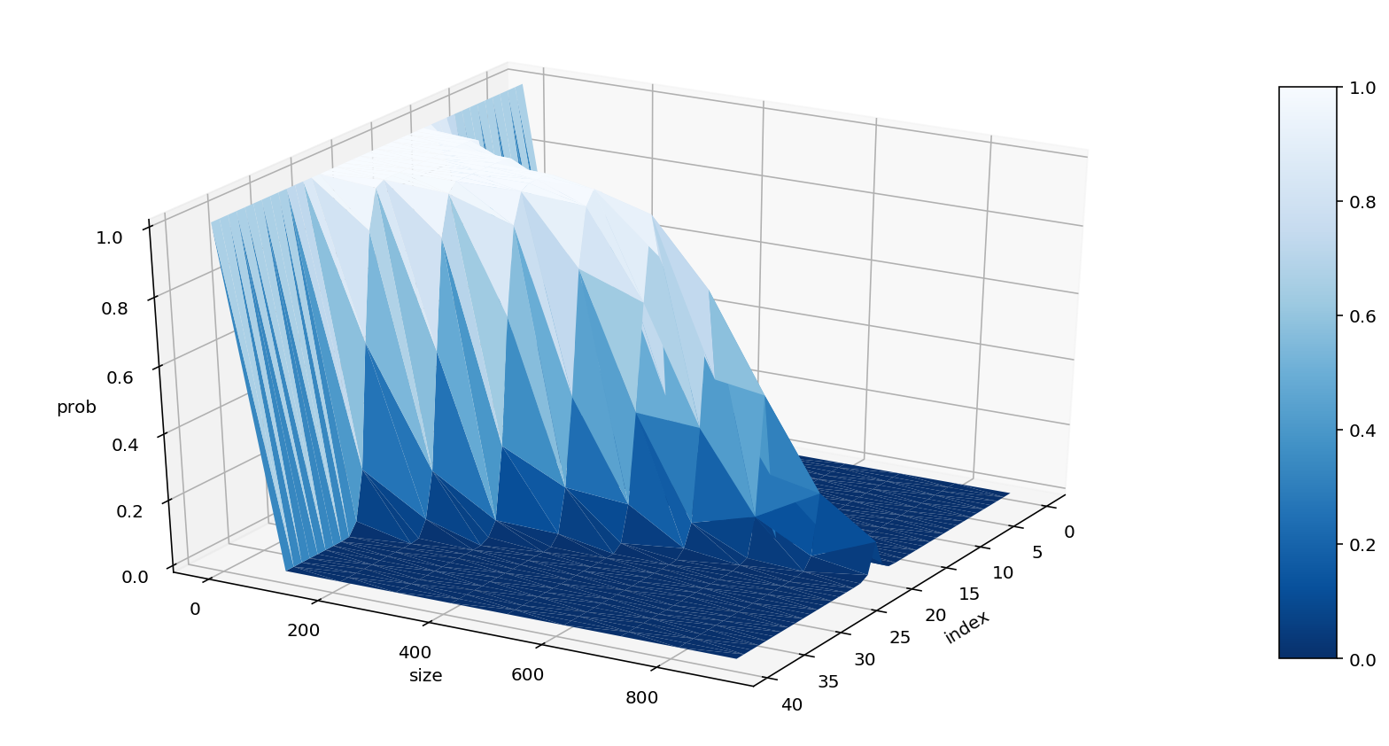
With this prediction procedure implemented, we can estimate the probability of our order (placed at the price bucket order_idx with size order_size) being executed within n_steps.

n_steps = 10
n_sim = 1000
order_idx = 12  # [0, 2n-1]
order_size = 100
success = 0
orderbook = np.zeros([1 + n_steps, 2 * n])
for i in range(n_sim):
    prediction = smm.smm.SMM.multivariate_t_rvs(S=S, m=m, df=7, n=n_steps)
    for j in range(1, n_steps + 1):
        orderbook[j, :n] = np.sort(orderbook[j - 1, :n] + prediction[j - 1, :n])[::-1]
        orderbook[j, n:] = np.sort(orderbook[j - 1, n:] + prediction[j - 1, n:])
    if orderbook[:, order_idx].min() + order_size <= 0:
        success += 1
success / n_sim

0.861

So a limit buy order at bid_8 ( $20 - 12 = 8$ ) with size 100 can be executed within 10 steps, at a probability of 86.1%. Moreover, we can even make a 3D surface plot to get a comprehensive idea of the whole distribution.

def evolve(order_idx, order_size, n_steps=10, n_sim=1000):
    success = 0
    orderbook = np.zeros([1 + n_steps, 2 * n])
    for i in range(n_sim):
        prediction = smm.smm.SMM.multivariate_t_rvs(S=S, m=m, df=7, n=n_steps)
        for j in range(1, n_steps + 1):
            orderbook[j, :n] = np.sort(orderbook[j - 1, :n] + prediction[j - 1, :n])[::-1]
            orderbook[j, n:] = np.sort(orderbook[j - 1, n:] + prediction[j - 1, n:])
        if orderbook[:, order_idx].min() + order_size <= 0:
            success += 1
    return success / n_sim


grid_idx = np.arange(0, 2 * n)
grid_size = np.arange(0, 1000, 100)
l_idx = len(grid_idx)
l_size = len(grid_size)
result = np.zeros([l_idx, l_size])
for i in range(l_idx):
    for j in range(l_size):
        result[i, j] = evolve(grid_idx[i], grid_size[j])


from mpl_toolkits.mplot3d import Axes3D
import seaborn as sns
 
# Transform data to a long format
data = pd.DataFrame(result, index=grid_idx, columns=grid_size)
df = data.unstack().reset_index()
df.columns = ['size', 'index', 'prob']
 
# Make the plot
fig = plt.figure(figsize=(12, 6))
ax = fig.gca(projection='3d')
surf=ax.plot_trisurf(df['index'], df['size'], df['prob'], cmap=plt.cm.Blues_r, linewidth=.1)
fig.colorbar(surf, shrink=.8, aspect=10)
ax.view_init(30, 30)
plt.tight_layout()
ax.set_xlabel('index')
ax.set_ylabel('size')
ax.set_zlabel('prob')
plt.show()

Reference

Rama Cont, Sasha Stoikov and Rishi Talreja. “A stochastic model for order book dynamics”. Operations Research, Volume 58, No. 3 (2010), 549-563.
David Peel, and Geoffrey J. McLachlan. “Robust mixture modelling using the t-distribution.” Statistics and computing 10, no. 4 (2000): 339-348.