The Perfect Market Maker: Is it Possible?

2019-04-23

In this research report we try to simulate and explore difference scenarios for a “perfect” market maker in the Bitcoin market. By “perfect” we refer to the capability to capture all spreads on the right side of any trade, i.e. there will be no spread loss at all. Although this setting is too perfect to be considered comparable with real trading, our analysis w.r.t. model parameters are believed to be insightful still.

Highlights

Self-explanatory backtest engine: the backtest engine is well encapsulated with limited public functions for people with little coding knowledge.
High-speed simulation: simulation per each set of parameters costs only ~2 ms without altering trading details.
Illustrated analysis: most analysis after parameter tuning is carried out with multiple (yet necessary) figures and elaborate explanation. Certain figures are made into animation for better understandability.

Dependencies

Import necessary modules and set up corresponding configurations. In this research notebook, we are using the following packages:

numpy: mathematical tools & matrix processing
pandas: data frame support
matplotlib: plotting
ipython: statistical analysis
numba: accelerating pure numerical calculation
ffmpeg: animation support (unnecessary for the rest of codes)

%config InlineB_smallackend.figure_format = 'retina'
import pandas as pd
import numpy as np
import matplotlib.pyplot as plt
import matplotlib.dates as mdates
from matplotlib.animation import FuncAnimation
from pandas.plotting import register_matplotlib_converters
from itertools import product
from time import time
from numba import njit
register_matplotlib_converters()
plt.style.use('bmh')
plt.rcParams['font.family'] = 'serif'
plt.rcParams['animation.html'] = 'html5'

Auxiliary Functions

In this section, several useful functions are introduced for later use during the backtest.

cumsum: It’s a modified version of the original cumulative summation function, the summation now handles two boundaries during calculation. Calculation is accelerated by JIT.
sharpe_ratio: It’s a handy function that calculates the annualized Sharpe ratio based on high-freq returns (returns are defined in percentage).
sortino_ratio: Similar as above, the function gives the annualized sortino ratio.

@njit
def cumsum(values, upper, lower):  # bounded cumsum
    '''
    PARAMS:
        values: numpy.array
        upper: float
        lower: float
    
    RETURN: numpy.array
    '''
    n = len(values)
    res = np.empty(n)
    sum_val = 0
    for i in range(n):
        x = min(max(sum_val + values[i], lower), upper)
        res[i] = x
        sum_val = x
    return res

def sharpe_ratio(rtn):  # calculate annualized sharpe ratio
    '''
    PARAMS:
        rtn: pandas.Series
    
    RETURN: float
    '''
    rtn = rtn.resample('H').sum()
    mean = rtn.mean()
    std = rtn.std()
    if std:
        return mean / std * np.sqrt(252 * 24)  # annualization
    else:
        return np.nan

def sortino_ratio(rtn):  # calculate annualized sortino ratio
    '''
    PARAMS:
        rtn: pandas.Series
    
    RETURN: float
    '''
    rtn = rtn.resample('H').sum()
    mean = rtn.mean()
    rtn.loc[rtn > 0] = 0
    downside_risk = rtn.std()
    if downside_risk:
        return mean / downside_risk * np.sqrt(252 * 24)  # annualize
    else:
        return np.nan

Backtest Engine

A backtest engine is designed for this problem.

Parameters

We have the following parameters (the first two are datasets) for simulation:

$s$ : target transaction size
$j$ : max long position (in Bitcoin)
$k$ : max short position (in Bitcoin)

Trade are participated only if:

The trade price is at the current best bid or offer price,
Trade quantity $q>4s$
The new position $x$ satisfies $−k \le x \le j$

Usage

be = BacktestEngine()
be.load(filename_Z='...', filename_B='...', root_dir='...')
be.run(s=..., j=..., k=...)

Specially, the class provides a great feature that prints the whole backtest process in an animation. In order to activate the feature, run command below

be.run(s=..., j=..., k=..., animation=True)

class BacktestEngine:
    def __init__(self):
        self.Z = None
        self.B = None
        self.__T = None
        self.__T_cached = {}
    
    def load(self, filename_Z, filename_B, root_dir='../', prog_bar=False):
        '''
        PARAMS:
            filename_Z: string
            filename_B: string
            root_dir: string (end with '/', default: '../')
        RETURN: (pandas.DataFrame, pandas.DataFrame)
        '''
        Z = pd.read_csv(root_dir + filename_Z, sep='\t')
        Z.columns = ['time', 'price', 'size']
        Z['time'] = pd.to_datetime(Z['time'], unit='us', utc=True)
        Z = Z.groupby(['time', 'price']).sum().reset_index()
        Z.set_index('time', inplace=True)
        Z = Z.tz_convert('America/Chicago').tz_localize(None)
        last_prices = Z.groupby(Z.index).price.transform(lambda _: _[-1])
        Z = Z[Z.price == last_prices]  # use the last price of same time
        self.Z = Z

        B = pd.read_csv(root_dir + filename_B, sep='\t')
        B.columns = [
            'ask1price', 'ask1size', 'ask2price', 'ask2size', 'ask3price', 'ask3size',
            'bid1price', 'bid1size', 'bid2price', 'bid2size', 'bid3price', 'bid3size',
            'time_recv', 'time'
        ]
        del B['time_recv']
        B['time'] = pd.to_datetime(B['time'], unit='us', utc=True)
        B.set_index('time', inplace=True)
        B = B.tz_convert('America/Chicago').tz_localize(None).sort_index()
        for i in (1, 2, 3):
            for s in ['ask', 'bid']:
                B[f'{s}{i}size'] /= 1e9
                B[f'{s}{i}price'] /= 1e6
        self.B = B
        
        B = B[['ask1price', 'bid1price']].copy()
        entries = []
        bi = 0
        n = len(Z)
        for i in range(n):
            if prog_bar: print('{:.2%}'.format((i + 1) / n), end='\r')
            p, q = z = Z.iloc[i]
            t = z.name
            while B.index[bi] <= t: bi += 1  # loop until book time > trade time
            a, b = B.iloc[bi - 1]  # use the last book before trade
            if p in (a, b):
                trade = -1 if p == a else 1
                mid = (a + b) / 2
                entries.append((t, p, q, trade, mid))
                
        T = pd.DataFrame(entries, columns=['time', 'price', 'volume', 'trade', 'mid'])
        T.set_index('time', inplace=True)  # set time as index
        self.__T = T
    
    def run(self, s, j, k, animation=False, fps=2, max_frames=200):
        '''
        PARAMS:
            s: float
            j: float
            k: float
            animation: boolean (default: False)
            fps: integer (default: 2)
            max_frames: integer (default: 200)
        
        RETURN: pandas.DataFrame | matplotlib.animation.FuncAnimation
        '''
        assert self.__T is not None
        if s not in self.__T_cached:
            self.__T_cached[s] = self.__T[self.__T.volume > 4 * s].copy()
        T = self.__T_cached[s].copy()
        T['position'] = cumsum(T.trade.values * s, upper=j - j % s, lower=k % s - k)
        T.trade = np.diff(T.position.values, prepend=0)
        # T = T[T.trade.abs() > 1e-12]
        T['cash'] = -(T.trade * T.price).cumsum()
        T['pnl'] = T.cash + T.position * T.mid
        if not animation: return T

        P = T.pnl.copy()
        Z = self.Z.copy()
        B = self.B.copy()

        P = P.resample('S').max().fillna(method='ffill')
        Z = Z.resample('S').max().fillna(method='ffill')
        B = B.resample('S').max().fillna(method='ffill')
        if len(B) > max_frames:
            frame_interval = np.ceil(len(B) / max_frames).astype(int)
            P = P.iloc[::frame_interval]
            Z = Z.iloc[::frame_interval]
            B = B.iloc[::frame_interval]
        c_xlim = P.index.min(), P.index.max()
        c_ylim = P.values.min(), P.values.max()
        c_range = c_ylim[1] - c_ylim[0]
        c_ylim = (c_ylim[0] - c_range / 4, c_ylim[1] + c_range / 4)
        t_xlim = Z.index.min(), Z.index.max()
        t_ylim = Z.price.min(), Z.price.max()
        p_range = t_ylim[1] - t_ylim[0]
        t_ylim = (t_ylim[0] - p_range / 4, t_ylim[1] + p_range / 4)
        b_ymax = B[[f'{s}{i}size' for i in (1, 2, 3) for s in ['ask', 'bid']]].max().max() * 1.05
        b_ylim = (0, b_ymax)
    
        fig = plt.figure(figsize=(12, 15))
        ax1 = fig.add_subplot(311)
        ax1.set_xlim(-0.5, 6.5)
        ax1.set_ylim(b_ylim)
        ax1.set_ylabel("Order Size")
        xlab = ("bid3", "bid2", "bid1", "", "ask1", "ask2", "ask3")
        ax1.set_xticks(range(7))
        ax1.set_xticklabels(xlab)
        colors = ("r", "r", "r", "k", "c", "c", "c")
        bars = plt.bar(range(7), [0] * 7, color=colors, align="center")
        ax2 = fig.add_subplot(312)
        line_a = ax2.plot([], [], "c-", label="ask price")[0]  # ask price
        line_m = ax2.plot([], [], "k-", label="Last price")[0]  # mid-price
        line_b = ax2.plot([], [], "r-", label="bid price")[0]  # bid price
        ax2.legend(frameon=False, loc="lower left")
        ax2.fmt_xdata = mdates.DateFormatter("%Y/%m/%d %H:%M:%S")
        ax2.set_xlim(t_xlim)
        ax2.set_ylim(t_ylim)
        ax2.set_ylabel("Price")
        ax3 = fig.add_subplot(313)
        line_c = ax3.plot([], [], "k-")[0]
        ax3.fmt_xdata = mdates.DateFormatter("%Y/%m/%d %H:%M:%S")
        ax3.set_xlim(c_xlim)
        ax3.set_ylim(c_ylim)
        ax3.set_ylabel('P&L')
        plt.close(fig)
    
        def animate(frame_no):
            bs = B.iloc[frame_no]
            bst = bs.name.to_pydatetime()
            t = Z[Z.index < bst]
            b = B[B.index < bst]
            c = P[P.index < bst]
            asks = [bs[f'ask{i}size'] for i in (1, 2, 3)]
            bids = [bs[f'bid{i}size'] for i in (3, 2, 1)]
            orders = bids + [0] + asks
            ax1.set_title(bst.strftime('%Y/%m/%d %H:%M:%S.%f')[:-3])
            for bar, order in zip(bars, orders):
                bar.set_height(order)
            line_m.set_data(t.index, t.price)
            line_b.set_data(b.index, b.bid1price - p_range / 100)  # offset for distinction
            line_a.set_data(b.index, b.ask1price + p_range / 100)
            line_c.set_data(c.index, c.values)
        
        frames = B.shape[0]
        interval = frames / fps
        anim = FuncAnimation(fig, animate, frames=frames, interval=interval, repeat=False)
        return anim

The BacktestEngine has been accelerated largely thanks to the vectorization and JIT features. Per each loop the calculation performance is shown as below (~2 ms per be.run).

be = BacktestEngine()
be.load(
    filename_Z='mkt_make_BTC_hw_small__trades.tab',
    filename_B='mkt_make_BTC_hw_small__book_lev_2.tab'
)

%timeit be.run(s=0.001, j=0.010, k=0.010)

2.11 ms ± 106 µs per loop (mean ± std. dev. of 7 runs, 100 loops each)

Preparatory Analysis

In this part we try to load a small dataset and compare our results against the one in reference. The order book is as below.

be = BacktestEngine()
be.load(
    filename_Z='mkt_make_BTC_hw_small__trades.tab',
    filename_B='mkt_make_BTC_hw_small__book_lev_2.tab'
)

be.B.head()

time	ask1price	ask1size	ask2price	ask2size	ask3price	ask3size	bid1price	bid1size	bid2price	bid2size	bid3price	bid3size
2018-04-08 17:08:00.246	7035.55	66.062339	7035.56	0.5	7035.57	1.50587	7035.54	5.582917	7035.53	0.00142	7035.5	0.011361
2018-04-08 17:08:01.426	7035.55	66.062339	7035.56	0.5	7035.57	1.50587	7035.54	5.584317	7035.53	0.00142	7035.5	0.011361
2018-04-08 17:08:08.293	7035.55	65.958939	7035.56	0.5	7035.57	1.50587	7035.54	5.584317	7035.53	0.00142	7035.5	0.011361
2018-04-08 17:08:08.437	7035.55	65.958939	7035.56	0.5	7035.57	1.50587	7035.54	5.570860	7035.53	0.00142	7035.5	0.011361
2018-04-08 17:08:08.485	7035.55	65.958939	7035.56	0.5	7035.57	1.50587	7035.54	5.591242	7035.53	0.00142	7035.5	0.011361

The trade data is as below.

be.Z.head()

time	price	size
2018-04-08 17:08:08.293	7035.55	0.1034
2018-04-08 17:08:13.472	7035.54	0.3900
2018-04-08 17:08:19.105	7035.55	0.1502
2018-04-08 17:08:20.858	7035.54	0.0630
2018-04-08 17:08:23.087	7035.54	0.1030

Now, the backtest result is as below. Here we use $s=0.01$ , $j=0.055$ and $k=0.035$ like in the reference. We conclude that our model is valid as the result coincides with the one given.

T = be.run(0.01, 0.055, 0.035)
T = T[T.trade != 0][['trade', 'cash', 'position']]
T

time	trade	cash	position
2018-04-08 17:08:08.293	-0.01	70.3555	-0.01
2018-04-08 17:08:13.472	0.01	0.0001	0.00
2018-04-08 17:08:19.105	-0.01	70.3556	-0.01
2018-04-08 17:08:20.858	0.01	0.0002	0.00
2018-04-08 17:08:23.087	0.01	-70.3552	0.01
2018-04-08 17:08:42.770	0.01	-140.7106	0.02
2018-04-08 17:08:47.415	0.01	-211.0660	0.03
2018-04-08 17:08:49.413	0.01	-281.4214	0.04
2018-04-08 17:08:51.663	0.01	-351.7768	0.05
2018-04-08 17:08:54.890	-0.01	-281.4213	0.04
2018-04-08 17:09:07.259	-0.01	-211.0658	0.03
2018-04-08 17:09:10.259	0.01	-281.4212	0.04
2018-04-08 17:09:14.027	0.01	-351.7766	0.05
2018-04-08 17:09:53.208	-0.01	-281.4866	0.04

Parameter Tuning

In this section, we opt for a simple grid search to find the best parameters of our strategy. There are several things to consider before we actually start searching.

Should we force $j=k$ ?

I believe the answer is yes. There is little reason we want to find the inter-relationship between the upper and lower bounds of our positions. Since we assume a short position yields direct cash out, we don’t distinguish between a long and a short trade really. Of course market may have its trend, but theoretically we don’t care about the result from searching on a $(j,k)$ grid.

Which metrics should we consider?

Like in most backtest scenarios, we use Sharpe and Sortino ratios as metrics. Besides these two, we also consider the final P&L as a crucial statistic here.

Hence, we run simulation on a $100\times 100$ grid of $(s,j=k)$ grid and keep track of outstanding results. Then we filter these results by the three metrics and keep only the best $10$ in all of the three.

be = BacktestEngine()
be.load(
    filename_Z='mkt_make_BTC_hw_big__trades.tab',
    filename_B='mkt_make_BTC_hw_big__book_lev_2.tab'
)

s_grid = np.arange(0.001, 0.101, 0.001)
jk_grid = np.arange(0.01, 1.01, 0.01)
nsim = len(jk_grid) * len(s_grid)

def record():  # keep track of results
    record.records = []
    def f(*args):
        record.records.append((*args,))
    return f

best_pnl = 0
best_sr = 0
best_st = 0
new_record = record()
start_time = time()
for i, (s, jk) in enumerate(product(s_grid, jk_grid)):
    prog = (i + 1) / nsim
    current_time = time()
    elapse = current_time - start_time
    eta = elapse / prog * (1 - prog)
    print('Running {} simulations: '
          'best_pnl={:.4f}, best_sr={:.4f}, best_st={:.4f} | '
          '{:.2%} finished, ETA={:.0f} s'
          .format(nsim, best_pnl, best_sr, best_st, prog, eta) + ' ' * 10, end='\r')

    j = k = jk
    params = (s, j, k)
    T = be.run(*params)
    if not T.shape[0]: continue
    pnl = T.pnl[-1]
    rtn = T.pnl.diff() / T.pnl.shift()  # calculate returns in percentage
    sr = sharpe_ratio(rtn)
    st = sortino_ratio(rtn)
    best_pnl = pnl if pnl > best_pnl else best_pnl
    best_sr = sr if sr > best_sr else best_sr
    best_st = st if st > best_st else best_st
    new_record(*params, pnl, sr, st)

Running 10000 simulations: best_pnl=366.5568, best_sr=14.1144, best_st=136.7319 | 100.00% finished, ETA=0 s

best_params = list(filter(lambda x: (np.nan not in x) and (min(x[-3:]) > 0),
                          record.records))
pnl_list, sr_list, st_list = list(zip(*best_params))[-3:]
best_params = [entries for _, _, _, entries in
               sorted(zip(pnl_list, sr_list, st_list, best_params))][-10:]

ndigits = int(np.ceil(np.log10(len(best_params))))
for i, entries in enumerate(best_params):
    print('(Record {:{ndigits}}) s={:.3f}, j={:.3f}, k={:.3f} | pnl={:7.4f}, sr={:7.4f}, st={:.4f}'
          .format(i, *entries, ndigits=ndigits))

(Record 0) s=0.006, j=0.780, k=0.780 | pnl=10.1482, sr= 0.0645, st=0.0905
(Record 1) s=0.005, j=0.690, k=0.690 | pnl=15.4882, sr= 5.8961, st=12.0982
(Record 2) s=0.006, j=0.830, k=0.830 | pnl=27.7178, sr= 5.4487, st=11.4175
(Record 3) s=0.005, j=0.790, k=0.790 | pnl=51.7044, sr= 5.9154, st=12.0906
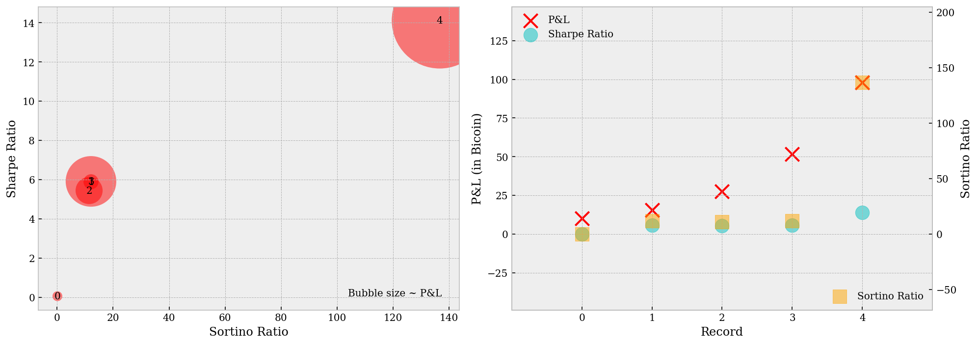
(Record 4) s=0.002, j=0.520, k=0.520 | pnl=97.8652, sr=14.1144, st=136.7319

The best parameters, together with their corresponding performance metrics, are plotted as below. The left plot shows the relative performance from record $0$ up to record $4$ (we filtered away most records as they give negative returns), which is a monotonic-like one and we have record $4$ an undoubtable winner. The right plot shows how our best $5$ sets of parameters differ from each other. Despite the total P&L is increasing, the Sharpe ratios hardly changes – this implies our search converged – or more possibly, end up overfitted.

def lim_generator(values, extend=.05):
    lower = min(values)
    upper = max(values)
    return lower * (1 + extend) - upper * extend, \
           upper * (1 + extend) - lower * extend

rec = np.arange(len(best_params))
pnl_list, sr_list, st_list = list(zip(*best_params))[-3:]

fig = plt.figure(figsize=(14, 5))

ax = fig.add_subplot(121)
# ax.set_xlim(lim_generator(st_list))
ax.set_ylim(lim_generator(sr_list))
sr_offset = (max(sr_list) - min(sr_list)) * 0.01
ax.scatter(st_list, sr_list, color='r', edgecolor='none', alpha=.5,
           s=(np.array(pnl_list) - min(pnl_list) + 10)**2 * 1)
ax.text(max(st_list) * 1.005, min(sr_list), 'Bubble size ~ P&L', ha='right')
for i, (st, sr) in enumerate(zip(st_list, sr_list)):
    ax.text(x=st, y=sr - sr_offset, s=str(i), ha='center')
ax.set_xlabel('Sortino Ratio')
ax.set_ylabel('Sharpe Ratio')

ax = fig.add_subplot(122)
ax.scatter(rec, pnl_list, color='r', marker='x', s=200, label='P&L')
ax.scatter(rec, sr_list, color='c', marker='o', s=200, alpha=.5, label='Sharpe Ratio')
ax.set_xlabel('Record')
ax.set_ylabel('P&L (in Bicoin)')
ax.set_ylim(lim_generator(np.concatenate([pnl_list, sr_list]), .5))
ax.legend(frameon=False, loc='upper left')
ax.xaxis.set_ticks(rec)
ax = ax.twinx()
ax.grid(None)
ax.scatter(rec, st_list, color='orange', marker='s', s=200, alpha=.5, label='Sortino Ratio')
ax.set_xlim(-1, len(best_params))
ax.set_ylabel('Sortino Ratio')
ax.set_ylim(lim_generator(st_list, .5))
ax.legend(frameon=False, loc='lower right')

plt.tight_layout()
plt.show()

Backtest Result

Before a thorough parameter analysis, we can also view the backtest performance in animation (ffmpeg required on your computer). It can be seen that our P&L has a rather similar trajectory comparing with the Bitcoin price, only that it’s direction of movement is opposite to the second. This implies we’re probably holding short positions most of the time.

be.run(*best_params[4][:3], animation=True)

Parameter Analysis

In this section, we try to take an overall look on the whole parameter grid as well as the outputs. Here are several questions we intend to answer by the end of this part:

Is is true that performance is monotonic w.r.t. $j$ (and $k$ )?

As we found in the previous section, with larger $j$ (and $k$ ) values we have higher P&L and ratios. We will investigate into this issue here. The two plots below gives some insight on this question. As we can tell from the left figure below, the best performance from larger $j$ (and $k$ ) values are indeed greater than those from smaller values, however, so are the worst results. This result coincides with the intuitive that larger position range means larger risk exposure over time, and therefore, more uncertainty in performance.

st001 = []
for entries in record.records[:100]:
    st001.append(entries[-1])
st005 = []
for entries in record.records[400:500]:
    st005.append(entries[-1])
st010 = []
for entries in record.records[900:1000]:
    st010.append(entries[-1])
st100 = []
for entries in record.records[9900:10000]:
    st100.append(entries[-1])

fig = plt.figure(figsize=(14, 5))
ax = fig.add_subplot(121)
ax.plot(jk_grid, st001, 'r', label='`$s=0.001$`')
ax.plot(jk_grid, st005, 'green', label='`$s=0.005$`')
ax.plot(jk_grid, st010, 'c', label='`$s=0.010$`')
ax.plot(jk_grid, st100, 'orange', label='`$s=0.100$`')
ax.legend(loc='upper left', frameon=False)
ax.set_xlabel('`$j$` (and `$k$`)')
ax.set_ylabel('Sortino Ratio')

ax = fig.add_subplot(122)
bins = np.linspace(-30, 20, 100)
ax.hist(st001, bins=bins, edgecolor='k', facecolor='r', alpha=.5, label='`$s=0.001$`')
ax.hist(st005, bins=bins, edgecolor='k', facecolor='green', alpha=.5, label='`$s=0.005$`')
ax.hist(st010, bins=bins, edgecolor='k', facecolor='c', alpha=.5, label='`$s=0.010$`')
ax.hist(st100, bins=bins, edgecolor='k', facecolor='orange', alpha=.5, label='`$s=0.100$`')
ax.set_xlabel('Sortino Ratio')
ax.legend(frameon=False)

plt.tight_layout()
plt.show()

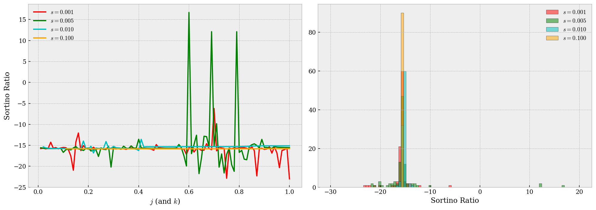
Does smaller $s$ yields better performance?

Similar as above, this guess is suggested from our grid search. First, from the right figure above we may tell that smaller $s$ yields a more volatile performance – by volatile, it means we have more chance to attain better results. In the contrast, larger values give significantly more robust (yet around a negative Sortino ratio) performance and thus we conclude smaller $s$ are more preferable.

Potential problems in the backtest?

There could be a lot of problems in fact, e.g. we are never a “perfect” market maker. But more severely, we may encounter some problem that we could’ve avoided, e.g. are we significantly biased to one side of trade, or, are we overfitting our model?

T = be.run(*record.records[4][:3])

fig = plt.figure(figsize=(14, 5))

ax = fig.add_subplot(121)
ax.scatter(T.index, T.position, color='r', s=1, alpha=.5)
ax.set_xlim(T.index.min(), T.index.max())
ax.set_xlabel('Time of Day')
ax.set_ylabel('Position')
plt.xticks(rotation=0, ha='center')

ax = fig.add_subplot(122)
ax.axvline(x=0, color='k', ls='--', alpha=.5)
ax.hist(T.position, bins=30, edgecolor='k', facecolor='c', alpha=.5, density=True)
ax.set_xlabel('Position')
ax.set_ylabel('Density')

plt.tight_layout()
plt.show()

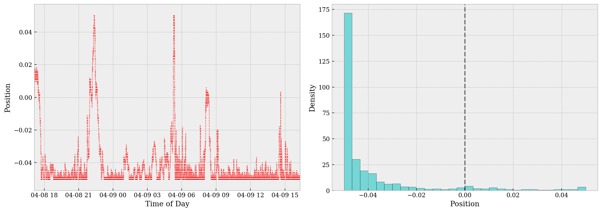
The two figures above shows the progress of our position over time. The position is, by and large, negative throughout the day. This can be infered either from the left scatter plot or from the right histogram (which is extremely biased to the left). The positive skewness in our position is a ruthless indication that we’ve overfit the model, mostly due to limitation of data. On such a small dataset, overfitting is highly risky and likely without cross-validatin methods etc. A potential cure for this may be using a larger dataset, or try to k-fold the timespan for CV.

In the meantime, let’s take a step back and analyze why the grid search gives us short position most time of the day. As far as I’m concerned, this is mainly because the profit we can obtain from taking a short position most of the time overwhelms that we can achieve from dynamic adjusting our side of trade and maintaining a neutral position. In a particular market like this given one where the general tendency of price is declining, a simple grid search ends up like this and we should’ve been aware of this before the whole analysis.

Numerically, the market making profit in this particular example is the price difference from each matched bid/ask and the corresponding mid price, which we used to calculate position market values. Under this setting, every trade we made we obtain a certain piece of revenue at no cost. The buy-and-hold profit, on the other hand, comes from holding a short position (in our story) and wait for the price to decline. We know the second profit is significantly larger than the first.

Theoretically, in order to fix this problem in its essence, we need to add one more parameter into our model, a parameter that rewards neutral positions or punishes holding a outstanding one. Available candidates include time-dollar product of a lasting position and moving averages of positions.

Conclusion

In this research, we tried to wrap up a simple backtest engine with a very special “perfect” market making setting. The setting is proved to be unrealistic but still provided a number of insights after detailed analysis. In the meantime, we may improve the model in a variety of ways based on the last sector Parameter Analysis.