Spread Trading: XOP and DRIP
2019-04-23
In this strategy we try to do spread trading based on the M-day (adjusted) returns of two highly related ETFs (exchange-traded funds). The intuition is to hedge the one-sided risks of buy-and-holding one specific ETF with (in expectation) increasing returns, by holding an opposite position of another ETF with decreasing returns. Once we have that the two ETFs’ returns are highly correlated, we can trade and make profit by this sort of pair trading.
Apart from M, we define trading thresholds g and j, together with stop-loss threshold s. Total capital limit K is assumed to be twice of N, namely the 15-day rolling median volume (of the less liquid ETF). Specifically, we first calculate the array of daily minimums of the two (adjusted) volume series, and then calculate the 15-day rolling median of this series as N. Apart from the capital limit, we also define daily position value (if any) based on N, which is N/100.
Specifically, for each trading day, we have workflow as below.
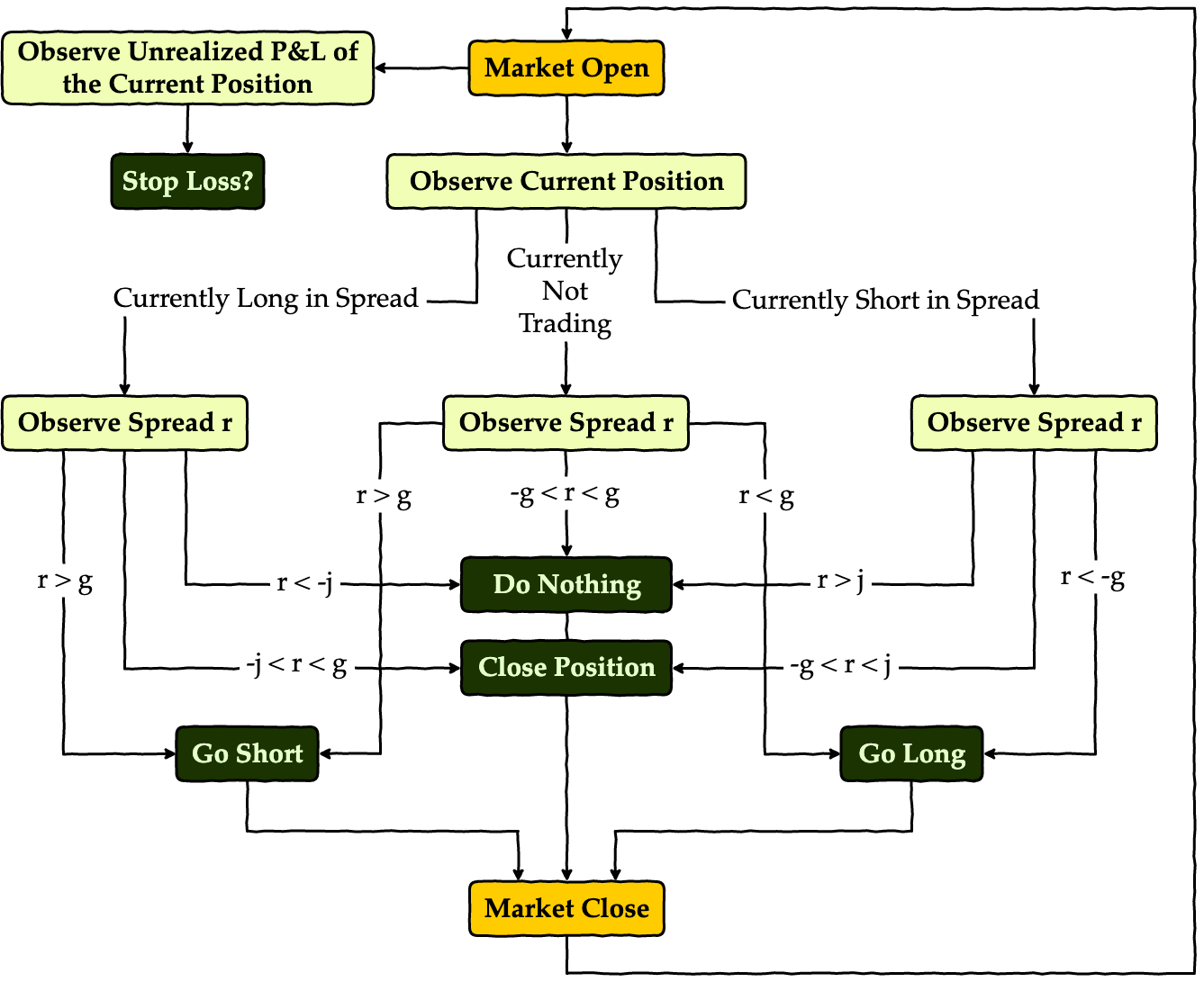
Apart from this process, we also keep track of our risk exposure with a stop-loss threshold, and try to do trading only within a month’s time, i.e. we start trading only when it’s the start of a new month, and kill any position every time it’s the end of a month.
Dependencies
Import necessary modules and set up corresponding configurations. In this research notebook, we are using the following packages:
- Quandl: source of financial data
- NumPy: mathematical tools & matrix processing
- Pandas: data frame support
- Matplotlib: plotting
- SciPy: statistical analysis
- StatsModels: statistical analysis
import warnings
import quandl
import numpy as np
import pandas as pd
import matplotlib.pyplot as plt
from scipy.stats import norm, t
from statsmodels.tsa.stattools import adfuller


pd.set_option('display.max_rows', 30)
plt.style.use('bmh')
plt.rcParams['font.family'] = 'serif'
plt.rcParams['font.size'] = 15
warnings.filterwarnings('ignore')
quandl.ApiConfig.api_key = QUANDL_API_KEY
Preparatory Analysis
In this part, we will try to analyze the economic and statistical features in the data. Here the two ETFs we’re using are XOP and DRIP. Data is retrieved from Quandl from 2015-12-02 to 2018-12-31. We’ll use only data from 2015-12-02 to 2016-12-01 for this section, as we don’t want to include future information during the backtest. Also, while it’s always better to have longer historical data for analysis, due to limited length of ETF data on Quandl (specifically for these two ETFs) we’re unfortunately restrained to this short timespan.
Definition of XOP
The SPDR S&P Oil & Gas Exploration & Production ETF (XOP) seeks to provide investment results that, before fees and expenses, correspond generally to the total return performance of the S&P Oil & Gas Exploration & Production Select Industry Index. See here for more detailed description.
Definition of DRIP
The Direxion Daily S&P Oil & Gas Exp. & Prod. Bull and Bear 3X Shares (DRIP) seek daily investment results, before fees and expenses, of 300% of the inverse, of the performance of the S&P Oil & Gas Exploration & Production Select Industry Index. See here for more detailed description.
Relationship of XOP and DRIP
By definition of the two ETFs, we expect DRIP to track -300% the daily return of XOP. This means the spread we should be tracking is, instead of the return difference between the two, the difference of -300% of M-day returns of XOP and the M-day returns of DRIP. Also, we are supposed to hold, if any, positions of these two ETFs in a ratio of XOP:DRIP = -3, no matter we’re long or short in the spread.
A peek into the data (assume M is 5.):
DRIP: price of DRIPXOP: price of XOPrDRIP: 5-day return of DRIPrXOP: 5-day return of XOPrXOPn3: -300% of 5-day return of XOPspread: spread ofrXOPn3fromrDRIP(spread = rDRIP - rXOPn3)
The first few entries of our data reads:
# exploratory settings
symbols = ('DRIP', 'XOP')
dates = ('2015-12-02', '2016-12-01')
M = 5

# retrieve data
df_X = quandl.get('EOD/' + symbols[0], start_date=dates[0], end_date=dates[1])
df_Y = quandl.get('EOD/' + symbols[1], start_date=dates[0], end_date=dates[1])
X = df_X.Adj_Close
Y = df_Y.Adj_Close

# calculate M-day returns
rX = (X.diff(M) / X.shift(M)).dropna()
rY = (Y.diff(M) / Y.shift(M)).dropna()
rY3 = rY * -3
spread = rX - rY3

# concat all variables
df = pd.concat([X, Y, rX, rY, rY3, spread], axis=1).dropna()
del X, Y, rX, rY, rY3, spread, df_X, df_Y
df.columns = [symbols[0], symbols[1],
              'r' + symbols[0], 'r' + symbols[1],
              'r' + symbols[1] + 'n3', 'spread']

df.head(10)
| Date | DRIP | XOP | rDRIP | rXOP | rXOPn3 | spread |
|---|---|---|---|---|---|---|
| 2015-12-09 | 93.228406 | 31.481858 | 0.300551 | -0.091874 | 0.275621 | 0.024930 |
| 2015-12-10 | 87.783600 | 32.033661 | 0.175401 | -0.063402 | 0.190207 | -0.014806 |
| 2015-12-11 | 100.660997 | 30.465377 | 0.247456 | -0.084908 | 0.254725 | -0.007269 |
| 2015-12-14 | 107.982471 | 29.719958 | 0.113006 | -0.041524 | 0.124571 | -0.011565 |
| 2015-12-15 | 101.685757 | 30.310485 | 0.065597 | -0.028545 | 0.085635 | -0.020037 |
| 2015-12-16 | 108.538063 | 29.632831 | 0.164217 | -0.058733 | 0.176199 | -0.011983 |
| 2015-12-17 | 118.711577 | 28.616350 | 0.352321 | -0.106679 | 0.320036 | 0.032284 |
| 2015-12-18 | 125.551661 | 28.154731 | 0.247272 | -0.075845 | 0.227535 | 0.019737 |
| 2015-12-21 | 130.267899 | 27.862871 | 0.206380 | -0.062486 | 0.187459 | 0.018921 |
| 2015-12-22 | 125.008291 | 28.203374 | 0.229359 | -0.069518 | 0.208553 | 0.020806 |
Also we may plot the histogram of the spread. Here we plot it against the fitted normal and t distributions. Apparently the t distribution matches our spread data better, which coincides with our expectation as financial data is commonly seen with fat tails. Also, we may notice that the spread is well centered around zero, which reassures us that we can assume symmetrical thresholds for trading.
fig = plt.figure(figsize=(20, 7.5))

ax = fig.add_subplot(121)
ax.hist(df.spread, bins=50, edgecolor='k', facecolor='c', density=True)
x_grid = np.linspace(-.2, .2, 200)

# fit to normal
params = norm.fit(df.spread)
pdf_fitted = norm.pdf(x_grid, *params)
plt.plot(x_grid, pdf_fitted, color='r',
         label='$\mathcal{N}$' + '({:.2f},{:.2f})'.format(*params))

# fit to t
params = t.fit(df.spread)
pdf_fitted = t.pdf(x_grid, *params)
plt.plot(x_grid, pdf_fitted, color='orange',
         label='t({:.2f},{:.2f},{:.2f})'.format(*params))

ax.set_xlabel('Spread')
ax.set_ylabel('Density')
ax.legend(frameon=False, loc='upper left')

ax = fig.add_subplot(122)
df.spread.plot(ax=ax, color='k')
plt.xticks(rotation=0, ha='center')
ax.set_xlabel('Date')
ax.set_ylabel('Spread')

plt.tight_layout()
plt.show()
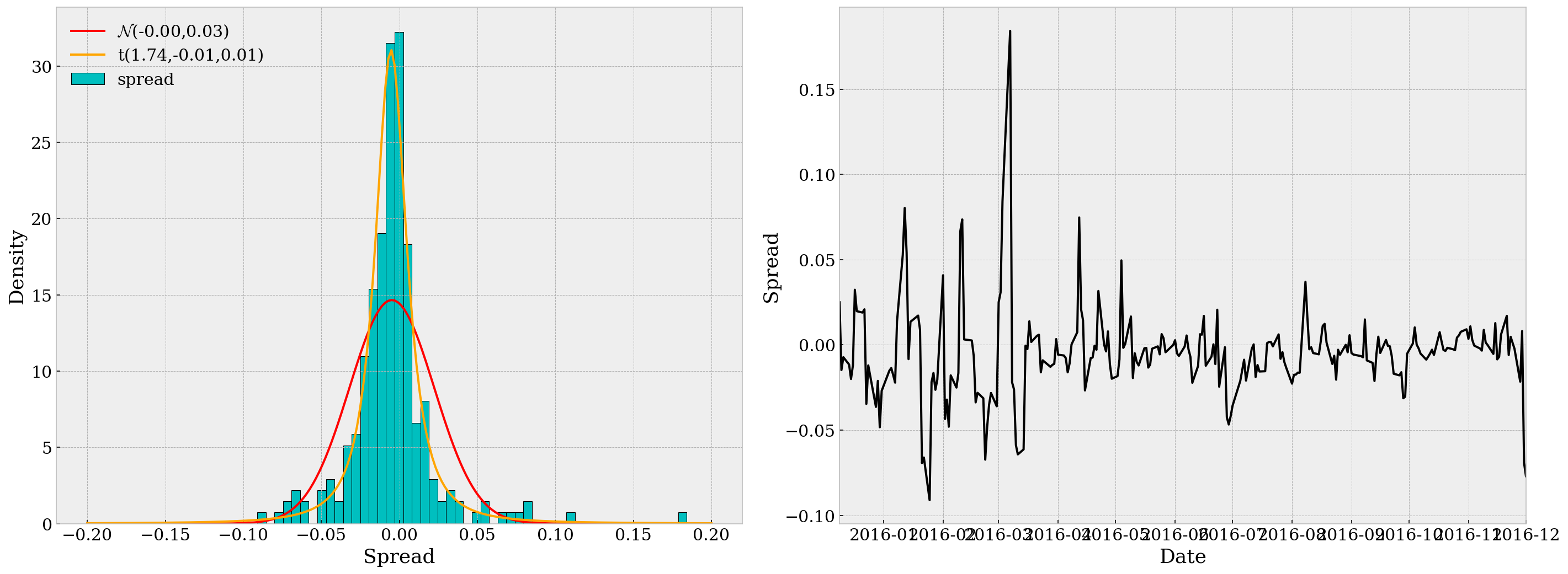
In the second subplot, we can see that the spread series is quite “stationary” over time, but we’d better not stop just observing by eye. (Also it’s a bit heteroskedastic, but we’re not focusing on that in this research.)
Statistical Tests
Below are some statistical tests we need to run through before actual pair traing. For detailed reasoning please refer to this post.
- Test for Unit Root: Here we use the Augmented Dickey-Fuller test. The p-value is 6.35e-14 $\ll$ 0.05, so we may safely reject the null.
result = adfuller(df.spread)
print('ADF Statistic: {}\np-value: {}\nCritical Values:'.format(*result[:2]))
for key, value in result[4].items():
    print('\t{}: {:.3f}'.format(key, value))
ADF Statistic: -8.614239430241229
p-value: 6.353844261802846e-14
Critical Values:
    1%: -3.458
    5%: -2.874
    10%: -2.573
- Test for Strong Stationarity: Here we opt for the Hurst Exponent. By definition, Hurst value H < 0.5 indicates the time series is mean-reverting, and our H value for the spread is -0.0390, so assumption is confirmed.
def hurst(ts):
    lags = range(2, 100)
    tau = [np.sqrt(np.std(np.subtract(ts[lag:], ts[:-lag]))) for lag in lags]
    poly = np.polyfit(np.log(lags), np.log(tau), 1)
    return poly[0]*2.0

np.random.seed(123)
gbm = np.log(np.cumsum(np.random.randn(100000))+1000)
mr = np.log(np.random.randn(100000)+1000)
tr = np.log(np.cumsum(np.random.randn(100000)+1)+1000)

print('H: {:.4f}'.format(hurst(df.spread)))
H: -0.0390
Based on the previous two test results we conclude our spread is mean-reverting and the strategy is reasonable.
Backtest Engine
In this part we design a simple backtest engine that takes ETF symbols, backtest timespan and the theoretical return ratio. It then provides an interface to run backtest against different parameters. I’ve encapsulated private methods/variables in the class BacktestEngine and there are only three attributes available:
BacktestEngine.symbols: tuple of ETF symbolsBacktestEngine.run: run backtest (returns Sortino ratio, Sharpe ratio, maximum drawdown and YoY return)BacktestEngine.df: stores the data from backtest (trade log)
The basic usage of this engine would be
be = BacktestEngine('DRIP', 'XOP', '2016-12-02', '2018-12-31', ratio=-3)
be.run(M=5, g=0.010, j=0.005, s=0.010, verbose=True)  # plot the backtest results
and if you want to check the tradelog during the timespan, call be.df. Note in this data frame, we denote the two ETFs by X and Y, and instead of the original M-day return of Y, we denote rY as ratio times the original M-day returns. The positions of X and Y are also reported in be.df together with daily and cumulative returns (in percentages of K).
An example of this be.df would be
| Date | X | Y | rX | rY | spread | N | pX | pY | daily_rtn | cum_rtn |
|---|---|---|---|---|---|---|---|---|---|---|
| 2016-12-22 | 12.267480 | 41.323160 | -0.019732 | -0.017567 | -0.002165 | 1.549400e+07 | 0 | 0 | 0.0 | 0.0 |
| 2016-12-23 | 12.208217 | 41.450761 | -0.017488 | -0.015711 | -0.001778 | 1.210184e+07 | 0 | 0 | 0.0 | 0.0 |
| 2016-12-27 | 12.000796 | 41.666701 | -0.018578 | -0.016343 | -0.002235 | 1.064284e+07 | 0 | 0 | 0.0 | 0.0 |
| 2016-12-28 | 12.445270 | 41.166112 | 0.003185 | 0.004286 | -0.001101 | 9.867562e+06 | 0 | 0 | 0.0 | 0.0 |
| 2016-12-29 | 12.692200 | 40.901094 | 0.017419 | 0.017180 | 0.000239 | 9.607867e+06 | 0 | 0 | 0.0 | 0.0 |
class BacktestEngine:

    def __init__(self, X_symbol, Y_symbol, start_date, end_date, ratio=1):
        '''
        PARAMETER:
            X_symbol: string
            Y_symbol: string
            start_date: string or datetime object
            end_date: string or datetime object

        RETURN: None
        '''

        self.symbols = (X_symbol, Y_symbol)
        self.__dates = (start_date, end_date)
        self.__stop_loss_dates = []
        self.__ratio = ratio

        # load data
        df_X = quandl.get('EOD/' + self.symbols[0],
                          start_date=self.__dates[0],
                          end_date=self.__dates[1])
        df_Y = quandl.get('EOD/' + self.symbols[1],
                          start_date=self.__dates[0],
                          end_date=self.__dates[1])
        self.__data = [df_X, df_Y]
        self.__trading = False

    def __process_data(self):  # prepare data to feed model
        '''
        PARAMETER: None

        RETURN: None
        '''

        df_X, df_Y = self.__data

        # generate price and volume series
        N_X = df_X.Adj_Volume * df_X.Adj_Close
        N_Y = df_Y.Adj_Volume * df_Y.Adj_Close
        N = pd.concat([N_X, N_Y], axis=1).min(axis=1).rolling(15).median()
        self.__K = N.max() * 2
        X = df_X.Adj_Close
        Y = df_Y.Adj_Close

        # calculate M-day returns
        M = self.__M
        rX = (X.diff(M) / X.shift(M)).dropna()
        rY = (Y.diff(M) / Y.shift(M)).dropna() * self.__ratio
        spread = rX - rY

        # concat all variables
        df = pd.concat([X, Y, rX, rY, spread, N], axis=1).dropna()
        del X, Y, rX, rY, spread, N
        df.columns = ['X', 'Y', 'rX', 'rY', 'spread', 'N']
        self.df = df

    def __update_params(self, M, g, j, s):  # update parameters of the model
        '''
        PARAMETER:
            M: integer
            g: float
            j: float
            s: float

        RETURN: None
        '''

        assert isinstance(M, (int, np.integer)) and (M > 0), \
               'parameter M should be a positive integer'
        assert -g < j < g, 'parameter j and g should follow -g < j < g'
        assert 0 < s, 'parameter s should be positive'

        self.__M = M
        self.__g = g
        self.__j = j
        self.__s = s
        self.__process_data()

    @staticmethod
    def __posval(position, price1, price2, gross=False):  # calculate value
        '''
        PARAMETER:
            position: float
            price1: float
            price2: float
            grodd: boolean (default: False)

        RETURN: float
        '''

        if gross:
            return abs(position[0]) * price1 + abs(position[1]) * price2
        else:
            return position[0] * price1 + position[1] * price2

    def __pos(self, value, X, Y, longX=True):  # calculate positions
        '''
        PARAMETER:
            value: float
            X: float
            Y: float
            longX: boolean (default: True)

        RETURN: (float, float)
        '''

        pX = round(value / X) * abs(self.__ratio)
        pY = round(value / Y) * (1 if self.__ratio > 0 else -1)
        return (pX, -pY) if longX else (-pX, pY)

    @staticmethod
    def __sharpe_ratio(daily_rtn):  # calculate sharpe ratio
        '''
        PARAMETER:
            daily_rtn: pd.Series of float

        RETURN: float
        '''

        return daily_rtn.mean() / daily_rtn.std()

    @staticmethod
    def __sortino_ratio(daily_rtn):  # calculate sortino ratio
        '''
        PARAMETER:
            daily_rtn: pd.Series of float

        RETURN: float
        '''
        daily_rtn = daily_rtn.copy()
        mean_rtn = daily_rtn.mean()
        daily_rtn.loc[daily_rtn > 0] = 0
        downside_risk = daily_rtn.std()
        return mean_rtn / downside_risk

    @staticmethod
    def __maximum_drawdown(value):  # maximum drawdown
        '''
        PARAMETER:
            value: pd.Series of float

        RETURN: (float, datetime, datetime)
        '''

        end = (value.cummax() / value).idxmax()
        start = (value.loc[:end]).idxmax()
        mdd = 1 - value[end] / value[start]
        return mdd, start, end

    def run(self, M, g, j, s, verbose=True):  # run backtest using parameters
        '''
        PARAMETER:
            M: integer
            g: float
            j: float
            s: float
            verbose: boolean (default: True)

        RETURN: None
        '''

        self.__update_params(M, g, j, s)

        pX = []
        pY = []  # positions
        rtn = []
        curr_position = (0, 0)
        curr_rtn = 0
        prev_day = 0
        prev_cost = 0
        prev_gross_cost = 0
        spread = 0
        for date in self.df.index:
            if date.day < prev_day:  # check start of new month
                daily_rtn = curr_rtn
                curr_position = (0, 0)
                prev_cost = 0
                prev_gross_cost = 0
                self.__trading = True

            elif self.__trading:  # trading (never stop-lossed this month)
                if curr_rtn < -self.__s * prev_gross_cost:  # stop loss
                    self.__stop_loss_dates.append(date)
                    daily_rtn = curr_rtn
                    curr_position = (0, 0)
                    prev_cost = prev_gross_cost = 0
                    self.__trading = False

                else:
                    if curr_position[0] > 1:  # currently long in X
                        daily_rtn = curr_rtn
                        if spread > self.__g:  # direactly from long to short
                            curr_position = self.__pos(N / 100, X, Y, False)
                            prev_cost = self.__posval(curr_position, X, Y)
                            prev_gross_cost = self.__posval(curr_position, X, Y, True)
                        elif spread > -self.__j:  # close position
                            curr_position = (0, 0)
                            prev_cost = prev_gross_cost = 0
                    elif curr_position[0] < -1:  # currently short in X
                        daily_rtn = curr_rtn
                        if spread < -self.__g:  # directly from short to long
                            curr_position = self.__pos(N / 100, X, Y, True)
                            prev_cost = self.__posval(curr_position, X, Y)
                            prev_gross_cost = self.__posval(curr_position, X, Y, True)
                        elif spread < self.__j:  # close position
                            curr_position = (0, 0)
                            prev_cost = prev_gross_cost = 0
                    else:  # currently having no position
                        daily_rtn = 0
                        if spread > self.__g:  # open short position
                            curr_position = self.__pos(N / 100, X, Y, False)
                            prev_cost = self.__posval(curr_position, X, Y)
                            prev_gross_cost = self.__posval(curr_position, X, Y, True)
                        elif spread < -self.__g:  # open long position
                            curr_position = self.__pos(N / 100, X, Y, True)
                            prev_cost = self.__posval(curr_position, X, Y)
                            prev_gross_cost = self.__posval(curr_position, X, Y, True)

            else:  # ceased until next month
                daily_rtn = 0

            spread, X, Y, N = self.df[['spread', 'X', 'Y', 'N']].loc[date]
            curr_rtn = self.__posval(curr_position, X, Y) - prev_cost

            pX.append(curr_position[0])
            pY.append(curr_position[1])
            rtn.append(daily_rtn)
            prev_day = date.day

        self.df['pX'] = pX
        self.df['pY'] = pY
        self.df['daily_rtn'] = rtn
        self.df.daily_rtn /= self.__K  # rtn is stored in %
        self.df['cum_rtn'] = self.df.daily_rtn.cumsum()
        sortino = self.__sortino_ratio(self.df.daily_rtn)
        sharpe = self.__sharpe_ratio(self.df.daily_rtn)
        mdd = self.__maximum_drawdown(self.df.cum_rtn + self.__K)[0]
        yoy_rtn = (1 + self.df.cum_rtn[-1])**(250 / self.df.shape[0]) - 1
        if verbose: self.__plot()
        return sortino, sharpe, mdd, yoy_rtn

    def __plot(self):  # plot backtest results
        '''
        PARAMETER: None

        RETURN: None
        '''

        fig = plt.figure(figsize=(20, 15))

        ax1 = fig.add_subplot(221)
        self.df.rX.plot(ax=ax1, label='X', alpha=.5, color='darkgreen')
        self.df.rY.plot(ax=ax1, label='Y', color='pink')
        ax1.set_ylabel('Returns')
        self.df.spread.plot(ax=ax1, label='spread', color='k')
        plt.xticks(rotation=0, ha='center')
        plt.legend(frameon=False, loc='upper right')

        ax2 = fig.add_subplot(222)
        self.df.spread.plot(ax=ax2, label='spread', color='k')
        ax2.plot((min(self.df.index), max(self.df.index)),
                 (self.__g, self.__g), 'c--', label='$\pm$g')
        ax2.plot((min(self.df.index), max(self.df.index)),
                 (self.__j, self.__j), 'r--', label='$\pm$j')
        ax2.plot((min(self.df.index), max(self.df.index)),
                 (-self.__g, -self.__g), 'c--')
        ax2.plot((min(self.df.index), max(self.df.index)),
                 (-self.__j, -self.__j), 'r--')
        ax2.set_ylabel('Spread')
        plt.xticks(rotation=0, ha='center')
        plt.legend(frameon=False)

        mdd, sd, ed = self.__maximum_drawdown(self.df.cum_rtn + self.__K)

        ax3 = fig.add_subplot(223)
        self.df.N.plot(ax=ax3, label='N', color='k')
        ax3.set_ylabel('Total Dollar Volumes')
        plt.legend(frameon=False, loc='upper left')
        plt.xticks(rotation=0, ha='center')
        ax3_ = ax3.twinx()
        self.df.pX.abs().plot(ax=ax3_, label='position', alpha=.5, color='r')
        ax3_.ticklabel_format(axis='y', style='sci', scilimits=(5, 5))
        ax3_.axvspan(xmin=sd, xmax=ed, ymin=0, ymax=1, color='grey', alpha=.5)
        ax3_.set_ylim(ymin=0)
        ax3_.set_ylabel('Daily Position (Long)')
        ax3.grid(False)
        plt.legend(frameon=False, loc='upper right')

        ax4 = fig.add_subplot(224)
        ax4.axvspan(xmin=sd, xmax=ed, ymin=0, ymax=1, color='grey', alpha=.5)
        (self.df.daily_rtn * 100).plot(ax=ax4, label='Daily Return (%)', color='c')
        (self.df.cum_rtn * 100).plot(ax=ax4, label='Cum. Return (%)', color='r')
        ax4.scatter(self.__stop_loss_dates,
                    self.df.cum_rtn.loc[self.__stop_loss_dates] * 100,
                    marker='x', color='k', label='', zorder=10)
        ax4.set_ylabel('Return (%)')
        plt.xticks(rotation=0, ha='center')
        plt.legend(frameon=False)

        plt.tight_layout()
        plt.show()
Here for illustration, we make a test run with parameters M=5, g=0.010, j=0.005 and s=0.01. The timespan, as required throughout the analysis, is set from 2016-12-02 to 2018-12-31 inclusive. The special meta parameter ratio is set to -3.
be = BacktestEngine('DRIP', 'XOP', start_date='2016-12-02', end_date='2018-12-31', ratio=-3)
st, sr, md, rt = be.run(M=5, g=0.02, j=0.01, s=0.01, verbose=True)
print('Sortino Ratio={:.4f}, Sharpe Ratio={:.4f}, Maximum Drawdown={:.4g}, YoY Return={:.2%}'
      .format(st, sr, md ,rt))
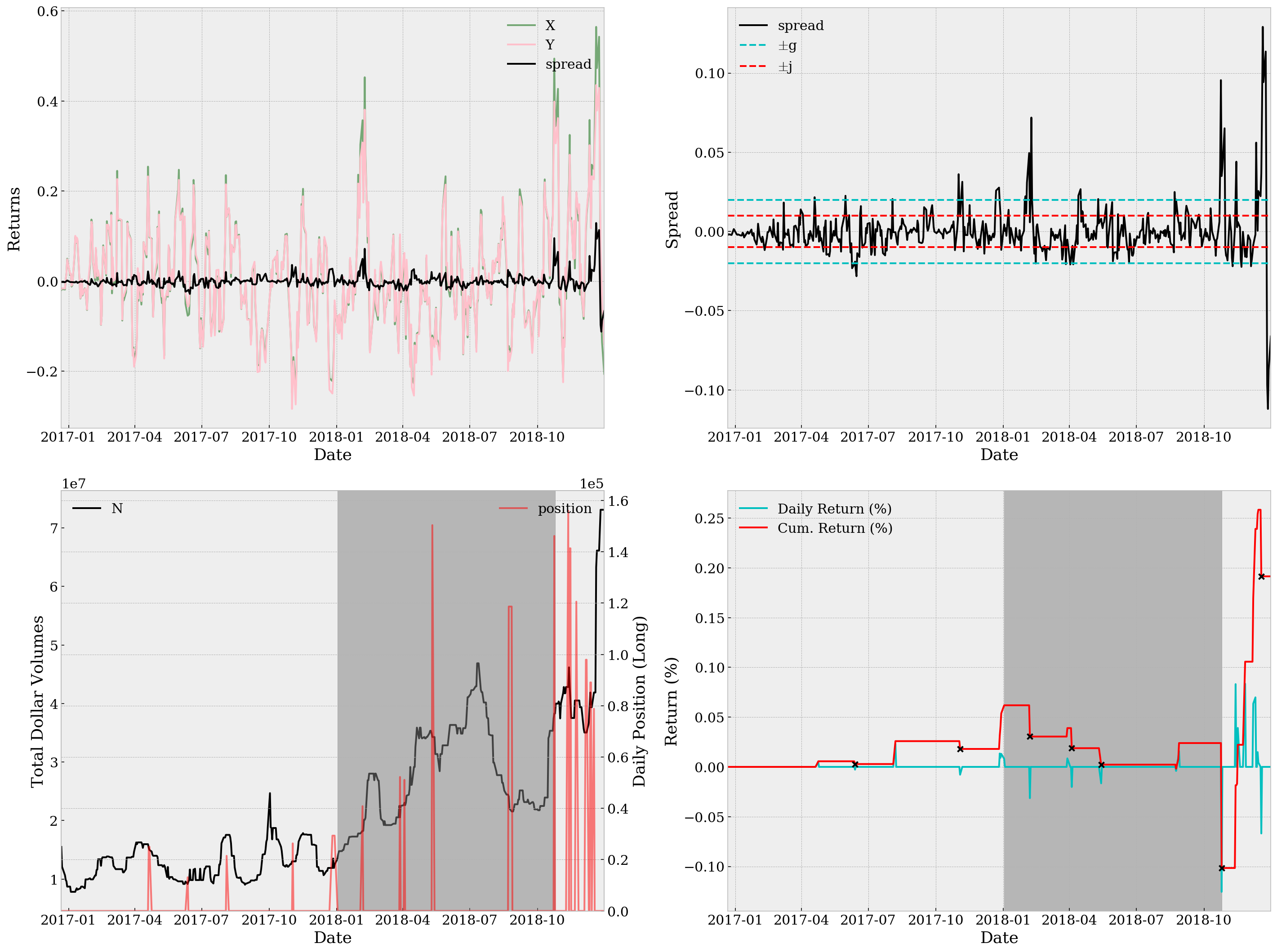
Sortino Ratio=0.0574, Sharpe Ratio=0.0387, Maximum Drawdown=1.118e-11, YoY Return=0.09%
With only a Sortino ratio of 0.0574, a Sharpe ratio of 0.0387 and YoY return of 0.09%, it’s definitely not a good strategy. Not to mention the unsatisfactory return plots. The top right subplot together with the bottom left one suggests that we might be using too wide thresholds. In case of detailed analysis, we can also take a look at be.df and specifically the trading days when we have non-zero positions, which turns out rather few (and supports our worry about wideness of thresholds):
be.df.loc[be.df.pX != 0]
| Date | X | Y | rX | rY | spread | N | pX | pY | daily_rtn | cum_rtn |
|---|---|---|---|---|---|---|---|---|---|---|
| 2017-04-20 | 19.072870 | 34.413981 | 0.191975 | 0.178984 | 0.012991 | 1.533244e+07 | -25014 | -4643 | 0.000000 | 0.000000 |
| 2017-04-21 | 18.845694 | 34.532005 | 0.097182 | 0.100743 | -0.003561 | 1.496846e+07 | -25014 | -4643 | 0.000011 | 0.000011 |
| 2017-06-12 | 21.522415 | 32.279704 | -0.076695 | -0.055866 | -0.020829 | 9.166219e+06 | 13122 | 2984 | 0.000000 | 0.000056 |
| 2017-08-04 | 22.747188 | 30.827585 | 0.142928 | 0.143423 | -0.000495 | 1.754893e+07 | -21483 | -5827 | 0.000000 | 0.000029 |
| 2017-11-02 | 15.319535 | 34.463445 | -0.210285 | -0.227637 | 0.017352 | 1.302198e+07 | -26349 | -3734 | 0.000000 | 0.000259 |
| 2017-12-26 | 11.398287 | 37.260895 | -0.221848 | -0.249496 | 0.027649 | 1.189655e+07 | -29352 | -3264 | 0.000000 | 0.000180 |
| 2017-12-27 | 11.645217 | 36.963916 | -0.200136 | -0.218041 | 0.017905 | 1.351392e+07 | -29352 | -3264 | 0.000135 | 0.000315 |
| 2017-12-28 | 11.418041 | 37.241096 | -0.152493 | -0.163117 | 0.010624 | 1.189655e+07 | -29352 | -3264 | 0.000092 | 0.000406 |
| 2017-12-29 | 11.714357 | 36.805528 | -0.054226 | -0.042553 | -0.011673 | 1.246303e+07 | -29352 | -3264 | 0.000131 | 0.000537 |
| 2018-02-05 | 14.331815 | 34.023830 | 0.357343 | 0.307833 | 0.049510 | 1.823786e+07 | -40842 | -5061 | 0.000000 | 0.000619 |
| 2018-03-28 | 13.193795 | 33.978894 | 0.097942 | 0.103973 | -0.006031 | 2.054748e+07 | 52227 | 6579 | 0.000000 | 0.000305 |
| 2018-04-03 | 12.630042 | 34.326023 | 0.045008 | 0.062801 | -0.017792 | 2.304128e+07 | 51093 | 6703 | 0.000000 | 0.000390 |
| 2018-05-11 | 7.140870 | 40.931377 | -0.120585 | -0.125726 | 0.005141 | 3.427444e+07 | -150390 | -8464 | 0.000000 | 0.000188 |
| 2018-08-23 | 6.237512 | 41.241724 | -0.144022 | -0.155054 | 0.011033 | 2.413513e+07 | -118650 | -5898 | 0.000000 | 0.000023 |
| 2018-08-24 | 6.039495 | 41.778234 | -0.157459 | -0.177582 | 0.020123 | 2.205453e+07 | -118650 | -5898 | -0.000041 | -0.000018 |
| 2018-08-27 | 5.960289 | 41.877588 | -0.146099 | -0.152580 | 0.006481 | 2.155575e+07 | -118650 | -5898 | 0.000098 | 0.000081 |
| 2018-10-24 | 9.096368 | 35.500295 | 0.494290 | 0.398785 | 0.095505 | 3.827526e+07 | -146172 | -9913 | 0.000000 | 0.000239 |
| 2018-11-12 | 9.106299 | 34.953065 | 0.168153 | 0.166935 | 0.001217 | 4.281623e+07 | 156027 | 11825 | 0.000000 | -0.001016 |
| 2018-11-14 | 9.801436 | 34.107346 | 0.324832 | 0.280804 | 0.044028 | 4.281623e+07 | -141351 | -13473 | 0.000000 | -0.000185 |
| 2018-11-15 | 9.364493 | 34.614778 | 0.136145 | 0.133480 | 0.002665 | 4.050823e+07 | -141351 | -13473 | 0.000016 | -0.000169 |
| 2018-11-23 | 11.211572 | 32.336311 | 0.197243 | 0.197471 | -0.000228 | 4.050823e+07 | 120567 | 12081 | 0.000000 | 0.000222 |
| 2018-12-06 | 11.797473 | 31.520441 | 0.111319 | 0.125227 | -0.013908 | 3.503895e+07 | 97920 | 10763 | 0.000000 | 0.001057 |
| 2018-12-07 | 11.906709 | 31.381147 | 0.147368 | 0.155996 | -0.008628 | 3.503895e+07 | 97920 | 10763 | 0.000635 | 0.001692 |
| 2018-12-12 | 12.989137 | 30.475730 | 0.209991 | 0.191626 | 0.018365 | 4.187946e+07 | -89073 | -12988 | 0.000000 | 0.002391 |
| 2018-12-13 | 13.187748 | 30.286687 | 0.117845 | 0.117424 | 0.000421 | 3.936253e+07 | -89073 | -12988 | 0.000148 | 0.002539 |
| 2018-12-17 | 16.375449 | 28.077868 | 0.248297 | 0.226081 | 0.022215 | 4.187946e+07 | -78804 | -13600 | 0.000000 | 0.002583 |
Parameter Tuning
As mentioned above, in this section we try to fit the best set of parameters from 2015-12-02 to 2016-12-01, i.e. the training set. As the focus of this report is not about efficient optimization, we opt for a simple grid search here. The parameter grids are defined as
M_grid: 5, 10, 15, 20 (4 in total)g_grid: 0.001, 0.003, …, 0.011 (6 in total)j_grid: -0.010, -0.008, …, 0.010 (11 in total)s_grid: 1e-3, 5e-3, 1e-2, 5e-2, 1e-1 (5 in total)
So no more than 1320 simulations are run. Note here parameter combinations where -g < j < g does not hold are neglected. Below are a selection of outstanding parameter sets during simulation.
from time import time
from itertools import product


def record():
    # record function with closure designed
    # to keep track of the best parameters
    record.best = []
    def f(*args):
        record.best.append((*args,))
    return f

mst, msr, mmd, mrt = 0, 0, 1, 0
M_grid = np.arange(5, 25, 5)
g_grid = np.arange(0.001, 0.012, 0.002)
j_grid = np.arange(-0.010, 0.011, 0.002)
s_grid = [1e-3, 5e-3, 0.01, 0.05, 0.10]
nsim = len(M_grid) * len(g_grid) * len(j_grid) * len(s_grid)
report_params = record()

be = BacktestEngine('DRIP', 'XOP', start_date='2015-12-02', end_date='2016-12-01', ratio=-3)

start_time = time()
for i, params in enumerate(product(M_grid, g_grid, j_grid, s_grid)):
    try:
        st, sr, md, rt = be.run(*params, verbose=False)
        if np.isnan(sr) or sr < 0 or st < 0: continue
        report = False
        if st > mst: mst, report = st, True
        if sr > msr: msr, report = sr, True
        if md < mmd: mmd, report = md, True
        if rt > mrt: mrt, report = rt, True
        prog = (i + 1) / nsim
        current_time = time()
        elapse = current_time - start_time
        eta = elapse / prog * (1 - prog)
        print('Running {} simulations... {:.2%} finished, ETA={:.0f}s'
              .format(nsim, prog, eta) + ' ' * 10, end='\r')
        if report: report_params(*params, st, sr, md, rt)
    except AssertionError:  # (-g < j < g) does not hold
        continue

st_list, sr_list, md_list, rt_list = list(zip(*record.best))[-4:]
record.best = [entries for _, entries in sorted(zip(st_list, record.best))][-5:]
record.best = [entries for _, entries in sorted(zip(sr_list, record.best))][-5:]
record.best = [entries for _, entries in sorted(zip(rt_list, record.best))][-5:]
record.best = [entries for _, entries in sorted(zip(md_list, record.best))][:5]

for i, entries in enumerate(record.best):
    print('(Record {:2}) M={:>2}, g={:.3f}, j={:6.3f}, s={:.5f},\t'
          'st={:.4f} sr={:.4f}, md={:9.4g}, rt={:6.2%}'
          .format(i, *entries))
(Record  0) M=15, g=0.007, j=-0.004, s=0.05000, st=1.4542 sr=0.3393, md=1.934e-10, rt= 8.99%
(Record  1) M=15, g=0.011, j=-0.010, s=0.05000, st=1.4591 sr=0.3430, md=1.673e-10, rt= 9.17%
(Record  2) M=20, g=0.007, j=-0.006, s=0.05000, st=1.5146 sr=0.3540, md=2.076e-10, rt= 9.47%
(Record  3) M=20, g=0.007, j= 0.006, s=0.05000, st=1.6001 sr=0.3534, md=  1.7e-10, rt= 9.33%
(Record  4) M=15, g=0.011, j=-0.004, s=0.05000, st=1.4680 sr=0.3452, md=1.673e-10, rt= 9.15%
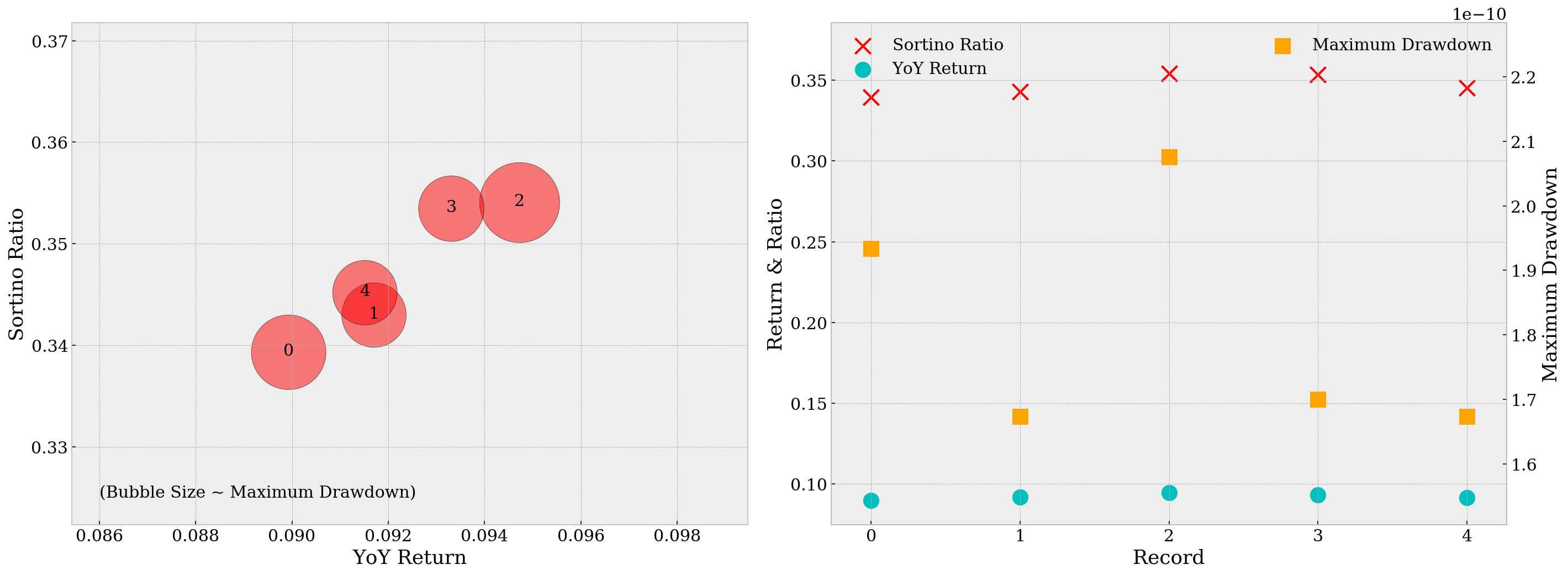
From the two plots below, we can tell that Record 3, or the parameter set M=20, g=0.007, j=0.006, s=0.05000, is a good choice as it has both large Sortino ratio/YoY return and a relatively small maximum drawdown. Record 2, or M=20, g=0.007, j=-0.006, s=0.05000 is also playing well among all outstanding parameter sets, with slightly better Sortino ratio and YoY returns but larger maximum drawdown. We’ll test on both sets.
rec = np.arange(len(record.best))
st_list, st_list, md_list, rt_list = list(zip(*record.best))[-4:]

fig = plt.figure(figsize=(20, 7.5))

ax = fig.add_subplot(121)
ax.set_xlim(min(rt_list) * 0.95, max(rt_list) * 1.05)
ax.set_ylim(min(st_list) * 0.95, max(st_list) * 1.05)
st_offset = (max(st_list) - min(st_list)) * 0.02
ax.scatter(rt_list, st_list, s=[(md / np.mean(md_list))**2 * 4e3 for md in md_list],
           color='r', edgecolor='k', alpha=.5)
ax.text(.086, .325, '(Bubble Size ~ Maximum Drawdown)')
for rt, st, i in zip(rt_list, st_list, range(len(record.best))):
    ax.text(x=rt, y=st - st_offset, s=str(i), ha='center')
ax.set_xlabel('YoY Return')
ax.set_ylabel('Sortino Ratio')

ax = fig.add_subplot(122)
ax.scatter(rec, st_list, color='r', marker='x', s=200, label='Sortino Ratio')
ax.scatter(rec, rt_list, color='c', marker='o', s=200, label='YoY Return')
ax.set_xlabel('Record')
ax.set_ylabel('Return & Ratio')
ax.legend(frameon=False, loc='upper left')

ax = ax.twinx()
ax.grid(False)
ax.scatter(rec, md_list, color='orange', marker='s', s=200, label='Maximum Drawdown')
ax.set_ylim(min(md_list) * 0.9, max(md_list) * 1.1)
ax.xaxis.set_ticks(rec)
ax.set_ylabel('Maximum Drawdown')
ax.legend(frameon=False, loc='upper right')

plt.tight_layout()
Using the parameters from Record 3, we run backtest against the test set, i.e. from 2016-12-02 to 2018-12-31. The plots are as below.
be = BacktestEngine('DRIP', 'XOP', start_date='2016-12-02', end_date='2018-12-31', ratio=-3)
st, sr, md, rt = be.run(M=20, g=0.007, j= 0.006, s=0.05000, verbose=True)
print('Sortino Ratio={:.4f}, Sharpe Ratio={:.4f}, Maximum Drawdown={:.4g}, YoY Return={:.2%}'
      .format(st, sr, md ,rt))
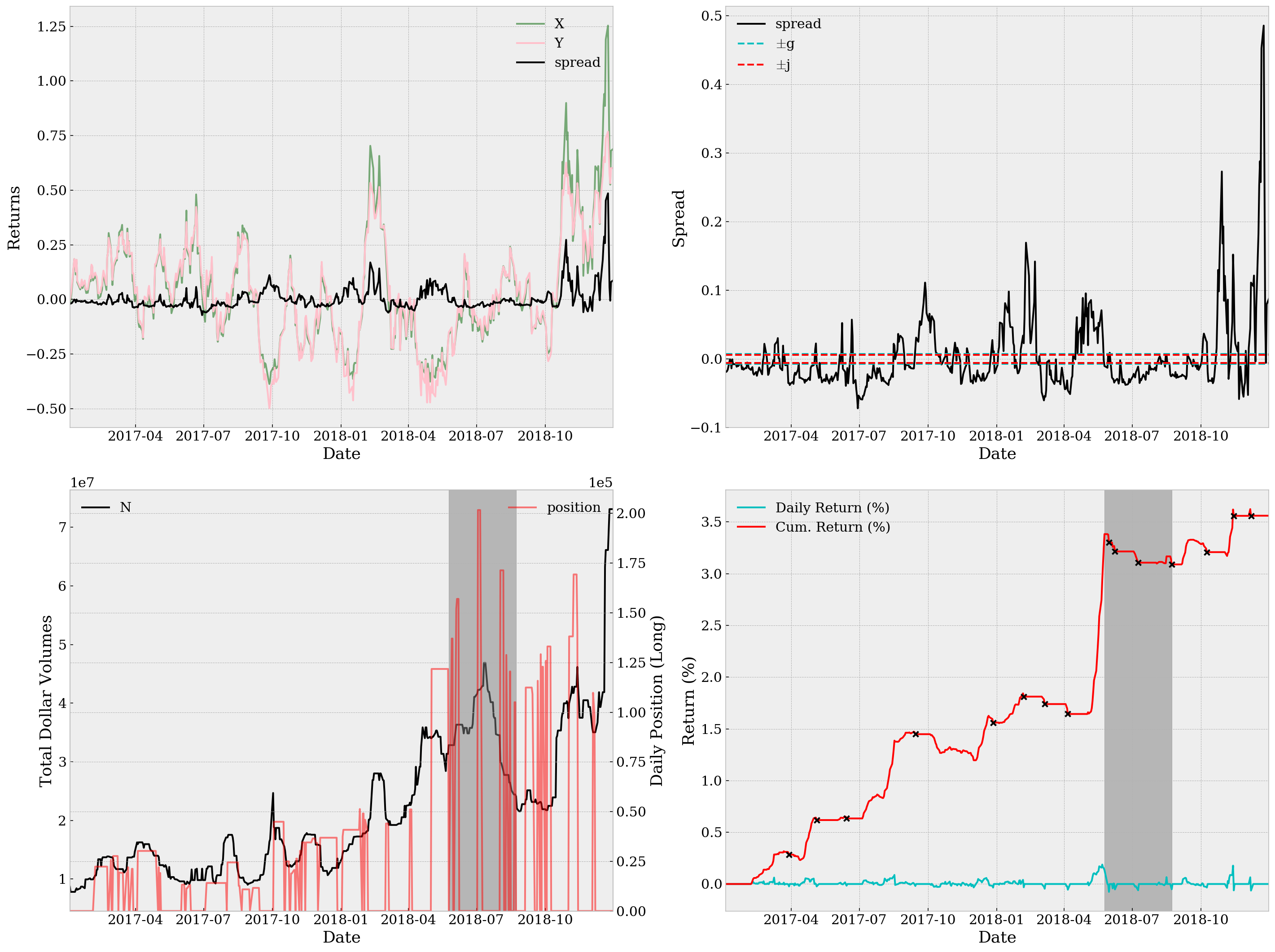
Sortino Ratio=0.7407, Sharpe Ratio=0.2447, Maximum Drawdown=2.005e-11, YoY Return=1.76%
Using the parameters from Record 3, the backtest result is as below.
be = BacktestEngine('DRIP', 'XOP', start_date='2016-12-02', end_date='2018-12-31', ratio=-3)
st, sr, md, rt = be.run(M=20, g=0.007, j=-0.006, s=0.05000, verbose=True)
print('Sortino Ratio={:.4f}, Sharpe Ratio={:.4f}, Maximum Drawdown={:.4g}, YoY Return={:.2%}'
      .format(st, sr, md ,rt))
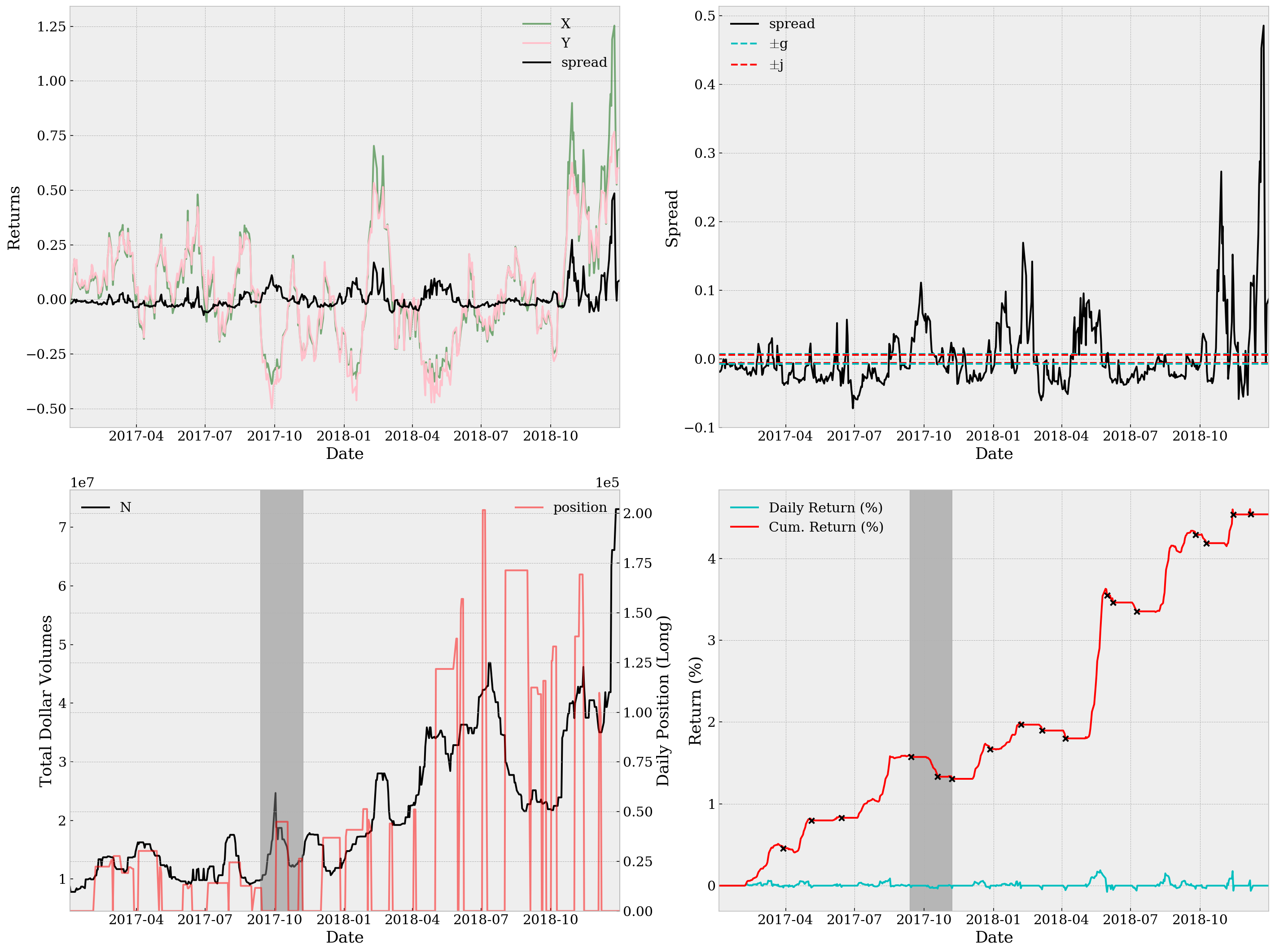
Sortino Ratio=0.9394, Sharpe Ratio=0.2872, Maximum Drawdown=1.997e-11, YoY Return=2.24%
Conclusion
Both results are amazingly great (especially compared with our result using random parameters before any tuning). Considering here we’re not utilizing any future data in backtest, the performance is satisfactory despite we’re neglecting a lot executional details in our analysis, like transaction costs and market impacts. There are also several comments on the processing of data:
- We are using the first
Mdays to calculate the rolling median ofN, which causes a loss in data. Perhaps we should useMdays of further previous historical data to make up this loss. - Thresholds change, over time. To be more specific, the “ideal” thresholds change all the time, partly due to market regime shifting and partly other unknown reasons. We may, therefore, never have the “best” parameters for trading. Should we go for a dynamic version of spread trading? I doubt so. But it’s worth thinking if there’s any remedy for this problem.