GMM Estimation of an ARMA(2,1) Model
2017-01-14
In econometrics and statistics, the generalized method of moments (GMM) is a generic method for estimating parameters in statistical models. Usually it is applied in the context of semiparametric models, where the parameter of interest is finite-dimensional, whereas the full shape of the data’s distribution function may not be known, and therefore maximum likelihood estimation is not applicable. Today, we are trying to write a Generalizd Method of Moments estimation framework in Python, and use it to estimate an ARMA(2,1) time series.
Model Description
Assume that now we have already determined the form of a time series model. It is
$$ X_t=\phi_1X_{t-1}+\phi_2X_{t-2}+\epsilon_t+\theta_1\epsilon_{t-1},\quad \epsilon_t\sim(0,1) $$
with at least 3 kinds of moment conditions given by
- The expectation residual:
$E(\epsilon_t)=0$ - The variance of the residual:
$E(\epsilon_t^2)=1$ - The covariance between
$\epsilon_s$and$\epsilon_t$($\forall s<t$):$Cov(\epsilon_s\epsilon_t)=0,\quad\forall s<t$
Now, assume we have a observed sample $x$ of the population $T$. Let the sample moment matrix be
where $k$ is the number of moment conditions. We define the sample mean of $g$ as $g_m(para, x_t)$:
$$ g_m(para)=\dfrac{1}{T}\sum_{t=1}^Tg(para,x_t) $$
Now, starting with the weight matrix $W_1=\mathbf{I}_{k\times k}$ we can proceed the iterated GMM estimation method as follows:
-
Minimize the objective function
$$ J(para)=Tg_m(para)^{\prime}W_ng_m(para) $$
and then solve for
$\widehat{para}_n$, that is$$ \widehat{para}_n=\underset{para}{\text{argmin }}J $$
-
Recompute
$W_n$based on the sample covariance of$g(\widehat{para}_n,x)$$$ S_n=\dfrac{1}{T}\sum_{t=1}^Tg(\widehat{para}_n,x)g(\widehat{para}_n,x)^{\prime} $$
$$ W_{n+1}=S_n^{-1} $$
-
Repeat step 1 and 2 until
$$ \left\Vert\widehat{para}_{n+1}-\widehat{para}_n\right\Vert<\delta $$
where
$\delta$is a given positive value that is very small. We may also terminate the iteration when reach an interation threshold.
Data Simulation
First we need to import some necessary Python libraries, including
- numpy for massive linear operations based on C,
- matplotlib for plotting,
- scipy for optimizing, and
- statsmodels in which there’re various built-in statistical models.
import numpy as np
import matplotlib.pyplot as plt
from scipy.optimize import minimize
import statsmodels.api as sm
from time import time
plt.rcParams['figure.figsize'] = (10,6)
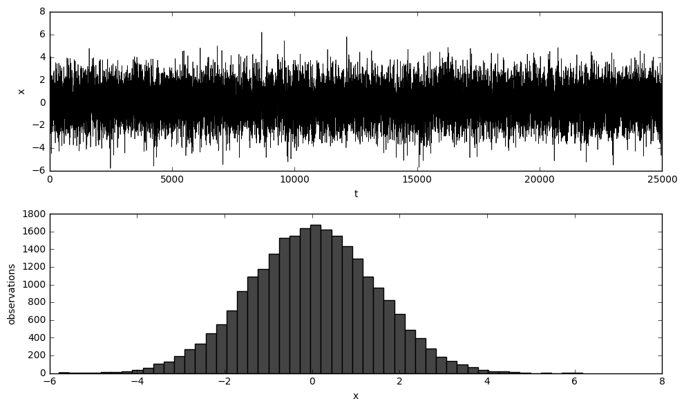
Here we define a function called simulate, which as its name implies, simulates a time series data determined by parameters $\phi_1$, $\phi_2$ and $\theta_1$. The initial values are given by init. The first 1/11 of the data are thrown away as burn-in, so that at last the sample size would be T. There is a built-in parameter called plot which is set True or 1 to plot the graph of the data, and False or 0 otherwise.
def simulate(T, phi, theta, init, plot=0):
    T = int(T)
    T_ = int(T * 1.1) # we will drop the first 1/11 observations here as burn-in
    X = np.ndarray(T_)
    X[0] = init[0]
    e = np.random.normal(0, 1, T_)
    for t in range(max(len(phi), len(theta)), T_):
        X[t] = sum([phi[i]*X[t-i-1] for i in range(len(phi))]) + \
               e[t] + \
               sum([theta[i]*e[t-i-1] for i in range(len(theta))])
    X = X[T_ - T:]    # burn-in
    if plot:          # plot the raw data
        plt.close()
        fig = plt.figure()

        ax1 = fig.add_subplot(211)
        ax1.set_xlim([0,T])
        ax1.plot(X, 'k-',lw=0.5)
        ax1.set_xlabel('t')
        ax1.set_ylabel('x')

        ax2 = fig.add_subplot(212)
        ax2.hist(X, color='#444444', bins=50)
        ax2.set_xlabel('x')
        ax2.set_ylabel('observations')

        plt.tight_layout()
        plt.show()
    return X
Now we can set the parameters and store them in separate lists.
# true parameters, initial entries and sample size
phi   = [0.2, 0.05]
theta = [0.8]
para  = np.array(phi + theta)
init  = [1, 1]
T     = 20000
T_    = T/4
We generate a time series dataset of size 5T/4, yet again we “set aside” the last T/4, so that we may compare the prediction of our estimation with the true data.
x = simulate(T + T_, phi, theta, init, plot=1)
x_true = x.copy()
x = x[:T] # We'll only use the first T observations to estimate parameters
GMM Estimation
Then we define a class named gmm, who has 2 major methods, namely fit and result. When we create an object (or model) of the class gmm, we initialize it with moment condition functions momn as well the jacobian of their mean w.r.t. the parameter vector, deriv_momn. When fitting our model to the data, we use the iterated gmm method, i.e. we alternately compute $\widehat{para}_n$ and weight matrix $W_n$, the major step of which undertaken by scipy’s minimize function, a brutal minimization method (with SLSQP method using jacobian matrix). The iteration terminates either when the square of the Euclidean distance between two estimators converges within a given value, $\delta$, or it reaches an iteration threshold (set at 10 here).
Remark 1: when iteration threshold is set at 2, this is immediately a 2-step GMM.
Remark 2: we here also estimate the asymptotic variance when fitting to the data. The derivation of this asymptotic variance estimation will be further discussed later.
class gmm():

    def __init__(self, momn, deriv_momn):
        self.n_momn     = len(momn)                                     # number of moment conditions
        self.n_para     = len(deriv_momn)                               # number of parameters
        self.momn       = momn                                          # moment conditions
        self.deriv_momn = deriv_momn                                    # derivative of the moment conditions
        self.para       = 2*np.random.rand(self.n_para)-1               # parameters, initialized at random

    def fit(self, x, plot=0):
        g  = lambda para: np.matrix([m(para, x) for m in self.momn])    # g is not a vector, but a matrix of the shape k * T
        gm = lambda para: np.mean(g(para), axis=1)                      # gm is a column vector
        J  = lambda para: np.asscalar(T * gm(para).T * W * gm(para))    # J is a scalar
        S  = lambda para: g(para) * g(para).T / T                       # S is the covariance matrix
        W  = np.identity(self.n_momn)                                   # W is the inverse of S
        jacobian   = lambda para: np.asarray(2 * T * gm(para).T * W * np.matrix([dm(para, x) for dm in self.deriv_momn]).T)
        iterations = 2                                                  # set 2 to make it a 2-step GMM

        if plot==1:
            print_len  = 14 * self.n_para + 4
            print(' '*((print_len-13)//2)+'GMM Iteration'+' '*((print_len-13)//2))
            print('='*print_len)
            print('No. Observations: {}'.format(T))
            print('='*print_len)
            print('Iter      {}'.format('        '.join(['para_{}'.format(i+1) for i in range(self.n_para)])))
            print('-'*print_len)

        cons = [{'type':'ineq','fun':lambda t: (1+t[i])*(1-t[i])} for i in range(self.n_para)]
        for i in range(iterations):
            temp = minimize(J, 2*np.random.rand(self.n_para)-1, method='SLSQP', constraints=cons, jac=jacobian).x
            temp /= max(np.abs(temp).max(), 1)
            delta = ((temp - self.para) ** 2).sum()
            if plot==1: print('\r{:>4}   {}   ({})'.format(i+1, '   '.join(['{: .4e}'.format(i) for i in temp]), delta), end='')
            if delta < 1e-10 or np.nan in temp: break
            self.para = temp
            W = np.linalg.inv(S(self.para))

        if plot == 1:
            print('\r{:>4}   {}   ({})'.format(i+1, '   '.join(['{: .4e}'.format(i) for i in self.para]), delta))
            print('-'*int(np.floor((print_len-3)/2))+'end'+'-'*int(np.ceil((print_len-3)/2)))

        g_star = lambda para: g(para) - gm(para)
        S_     = lambda para: g_star(para) * g_star(para).T / T
        avar   = np.linalg.inv(np.matrix([dm(self.para, x) for dm in self.deriv_momn]) * \
                               np.linalg.inv(S_(self.para)) * \
                               np.matrix([dm(self.para, x) for dm in self.deriv_momn]).T).diagonal().tolist()[0]

        self.J = J
        self.x = x
        self.avar = avar

    def result(self, para_true):
        print('{:^46}'.format('Iterated GMM Results'))
        print('='*46)
        print('Kind      {}'.format('        '.join(['para_{}'.format(i+1) for i in range(self.n_para)])))
        print('-'*46)
        print('Estm   {}'.format('   '.join(['{: .4e}'.format(i) for i in self.para])))
        print('True   {}'.format('   '.join(['{: .4e}'.format(i) for i in para_true])))
        print('-'*46)
        print('Avar   '+'   '.join('{: .4e}'.format(v) for v in self.avar))
        print('-'*46)
Below we define the moment condition functions and the derivatives of their mean.
momn = [lambda para, x: (x[4:] - para[0] * x[3:-1] - para[1] * x[2:-2]),  # expectation
        lambda para, x: (x[4:] - para[0] * x[3:-1] - para[1] * x[2:-2])**2 - (1 + para[2]**2),  # variance
        lambda para, x: (x[4:] - para[0] * x[3:-1] - para[1] * x[2:-2]) * \
                        (x[3:-1] - para[0] * x[2:-2] - para[1] * x[1:-3]) - para[2],  # covariance of epsilon_t and epsilon_{t-1}
        lambda para, x: (x[4:] - para[0] * x[3:-1] - para[1] * x[2:-2]) * \
                        (x[2:-2] - para[0] * x[1:-3] - para[1] * x[0:-4]),  # covariance of epsilon_t and epsilon_{t-2}
       ]

deriv_momn = [lambda para, x: np.array([(-x[3:-1]).mean(),
                                        (-2 * x[3:-1] * (x[4:] - para[0] * x[3:-1] - para[1] * x[2:-2])).mean(),
                                        (-x[3:-1] * (x[3:-1] - para[0] * x[2:-2] - para[1] * x[1:-3]) - x[2:-2] * \
                                         (x[4:] - para[0] * x[3:-1] - para[1] * x[2:-2])).mean(),
                                        (-x[3:-1] * (x[2:-2] - para[0] * x[1:-3] - para[1] * x[0:-4]) - x[1:-3] * \
                                         (x[4:] - para[0] * x[3:-1] - para[1] * x[2:-2])).mean(),
                                       ]),
              lambda para, x: np.array([(-x[2:-2]).mean(),
                                        (-2 * x[2:-2] * (x[4:] - para[0] * x[3:-1] - para[1] * x[2:-2])).mean(),
                                        (-x[2:-2] * (x[3:-1] - para[0] * x[2:-2] - para[1] * x[1:-3]) - x[1:-3] * \
                                         (x[4:] - para[0] * x[3:-1] - para[1] * x[2:-2])).mean(),
                                        (-x[2:-2] * (x[2:-2] - para[0] * x[1:-3] - para[1] * x[0:-4]) - x[0:-4] * \
                                         (x[4:] - para[0] * x[3:-1] - para[1] * x[2:-2])).mean(),
                                       ]),
              lambda para, x: np.array([0,
                                        -2 * para[2],
                                        -1,
                                        0,
                                       ])
             ]
Initialize the gmm model with moment condition functions and the respective partial derivatives, fit it to x, and then print out the result.
model = gmm(momn, deriv_momn)
model.fit(x, plot=1)
print()
model.result(para)
                GMM Iteration
==============================================
No. Observations: 20000
==============================================
Iter      para_1        para_2        para_3
----------------------------------------------
   2    1.9091e-01    5.6302e-02    8.1460e-01   (1.074866238949949e-08)
---------------------end----------------------

             Iterated GMM Results
==============================================
Kind      para_1        para_2        para_3
----------------------------------------------
Estm    1.9091e-01    5.6302e-02    8.1460e-01
True    2.0000e-01    5.0000e-02    8.0000e-01
----------------------------------------------
Avar    1.9905e+01    9.1790e+00    2.5171e+01
----------------------------------------------
As comparison, check the maximum likelihood estimation with the help of statsmodels.
print(sm.tsa.ARMA(x, (len(phi), len(theta))).fit().summary())
                              ARMA Model Results
==============================================================================
Dep. Variable:                      y   No. Observations:                20000
Model:                     ARMA(2, 1)   Log Likelihood              -28404.025
Method:                       css-mle   S.D. of innovations              1.001
Date:                Mon, 16 Jan 2017   AIC                          56818.050
Time:                        11:55:46   BIC                          56857.568
Sample:                             0   HQIC                         56830.979

==============================================================================
                 coef    std err          z      P>|z|      [95.0% Conf. Int.]
------------------------------------------------------------------------------
const          0.0026      0.017      0.155      0.876        -0.031     0.036
ar.L1.y        0.1983      0.010     20.706      0.000         0.179     0.217
ar.L2.y        0.0512      0.009      5.672      0.000         0.033     0.069
ma.L1.y        0.8050      0.006    128.761      0.000         0.793     0.817
                                    Roots
=============================================================================
                 Real           Imaginary           Modulus         Frequency
-----------------------------------------------------------------------------
AR.1            2.8895           +0.0000j            2.8895            0.0000
AR.2           -6.7643           +0.0000j            6.7643            0.5000
MA.1           -1.2423           +0.0000j            1.2423            0.5000
-----------------------------------------------------------------------------
Theoretical Asymptotic Variances of the GMM Estimator
Some assumptions:
and
where $e_t\in\mathbb{R}^{T\times1}$ is the $t^th$ basis vector. Hence,
where
and
$$ \mathcal{E}_3 = \begin{bmatrix} 0\ -2\theta_1\ -1\ 0 \end{bmatrix}. $$
Let
Since
$$ \mu = 0 $$
and the autocovariances $\gamma_i$ follows
$$ \begin{cases} \gamma_0-\phi_1\gamma_1-\phi_2\gamma_2=\theta_1(\phi_1+\theta_1)+1\ \phi_1\gamma_0+(\phi_2-1)\gamma_1=-\theta_1\ \gamma_k = \phi_1\gamma_{k-1} + \phi_2\gamma_{k-2},\quad k\ge 2 \end{cases} $$
we may derive $G$ at last.
Also, the covariance matrix of $e_t'g$ is
Now with $G$ and $S$, since
$$ \sqrt{T}\ (\widehat{para} - para)\overset{d}{\to}\mathcal{N}(0,(G’S^{-1}G)^{-1}), $$
we may derive the theoretical asymptotic variances of $\sqrt{T}\ \widehat{para}$ as follows.
mu = 0 # 345112251_00121231
A = np.matrix([[1,      -phi[0],  -phi[1]],
               [phi[0], phi[1]-1, 0],
               [phi[1], phi[0],   -1]
              ])
B = np.matrix([[theta[0]*(phi[0]+theta[0])+1],
               [-theta[0]],
               [0]
              ])
y = np.linalg.inv(A)*B
y0, y1, y2 = [np.asscalar(a) for a in y]
y3 = phi[0]*y2 + phi[1]*y1
y4 = phi[0]*y3 + phi[1]*y2
G = np.matrix([[-mu,                                     -mu,                                    0],
               [2*phi[0]*y0+2*(phi[1]-1)*y1,             2*phi[1]*y0+2*phi[0]*y1-2*y2,           -2*theta[0]],
               [(phi[1]-1)*y0+2*phi[0]*y1+(phi[1]-1)*y2, phi[0]*y0+(2*phi[1]-1)*y1+phi[0]*y2-y3, -1],
               [(phi[1]-1)*y1+2*phi[0]*y2+(phi[1]-1)*y3, -y0+phi[0]*y1+2*phi[1]*y2+phi[0]*y3-y4, 0]
              ])
G.round(2)
array([[ 0. ,  0. ,  0. ],
       [-1.6, -0. , -1.6],
       [-1.8, -0.8, -1. ],
       [-1.2, -1.8,  0. ]])
S = np.matrix([[1+theta[0]**2, 0,                             0,                           0],
               [0,             2*theta[0]**4+4*theta[0]**2+2, 2*theta[0]**3+2*theta[0],    0],
               [0,             2*theta[0]**3+2*theta[0],      theta[0]**4+3*theta[0]**2+1, theta[0]**3+theta[0]],
               [0,             0,                             theta[0]**3+theta[0],        theta[0]**4+2*theta[0]**2+1],
              ])
S.round(2)
array([[ 1.64,  0.  ,  0.  ,  0.  ],
       [ 0.  ,  5.38,  2.62,  0.  ],
       [ 0.  ,  2.62,  3.33,  1.31],
       [ 0.  ,  0.  ,  1.31,  2.69]])
np.linalg.inv(G.T*np.linalg.inv(S)*G).diagonal().tolist()[0]
[21.3174392361111, 9.980590277777774, 26.878064236111097]
model.avar
[19.905472617664184, 9.178999415080208, 25.170769966198534]
The estimated asymptotic variance is quite close to the theory.
Monte Carlo Simulation
Below we use the true parameters to simulate $N=10000$ times and each time we estimate a $\widehat{para}_n$.
N = 1000
para_mc = []
with np.errstate(divide='ignore'):
    start = time()
    for i in range(N):
        x_mc = simulate(T + T_, phi, theta, init)[:T]
        model.fit(x_mc)
        pct = i * 100 // N + 1
        now = time()
        eta = (100 - pct) / pct * (now - start)
        print('\r{:>3}% |'.format(pct)+'\u2591'*pct+' '*(100-pct)+'| ETA: {} s'.format(int(eta)), end='')
        para_mc.append(model.para)
print('\r100% |'+'\u2591'*100+'| Finished.', end='')
para_mc = np.array(para_mc)
100% |░░░░░░░░░░░░░░░░░░░░░░░░░░░░░░░░░░░░░░░░░░░░░░░░░░░░░░░░░░░░░░░░░░░░░░░░░░░░░░░| Finished.
plt.close()
fig = plt.figure()
ax1 = fig.add_subplot(311); ax1.hist(para_mc[:,0],bins=50,color='#444444',label='para[0]'); ax1.legend()
ax2 = fig.add_subplot(312); ax2.hist(para_mc[:,1],bins=50,color='#444444',label='para[1]'); ax2.legend()
ax3 = fig.add_subplot(313); ax3.hist(para_mc[:,2],bins=50,color='#444444',label='para[2]'); ax3.legend()
plt.tight_layout()
plt.show()
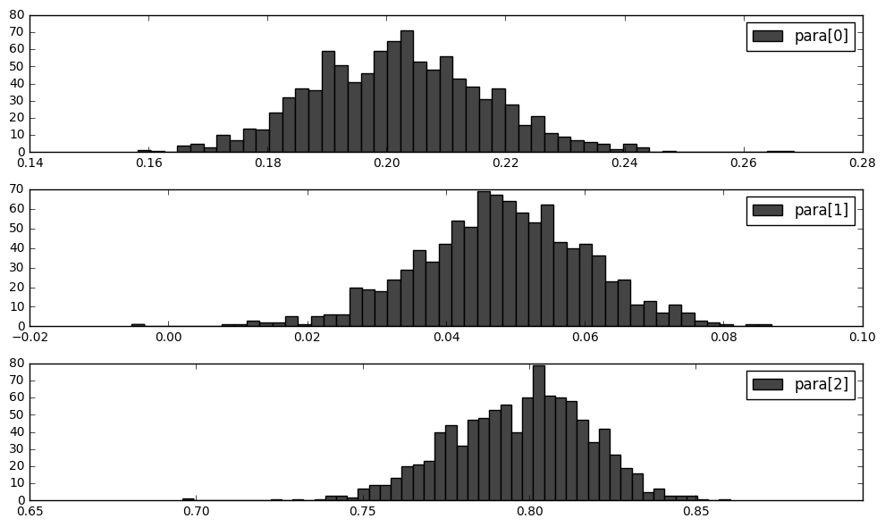
(para_mc.var(axis=0)*T).tolist()
[4.422402990203701, 2.9904249354938632, 8.796234771820194]
As we can see, the sample variance of the Monte Carlo simulated distribution of our estimator, is significantly smaller than the theoretical one. This should be a problem.
References:
- Hall, Alastair R. Generalized method of moments. Oxford University Press, 2005.
- Hall, Alastair R. “Hypothesis testing in models estimated by GMM.” Generalized method of moments estimation 5 (1999): 96.
- Hansen, Lars Peter. “Large sample properties of generalized method of moments estimators.” Econometrica: Journal of the Econometric Society (1982): 1029-1054.
- Wooldridge, Jeffrey M. “Applications of generalized method of moments estimation.” The Journal of Economic Perspectives 15.4 (2001): 87-100.